library(tidyverse)
library(tidytext)
library(forcats)
library(scales)

sentences <- data_frame(sentence = 1:3,
                text = c("I just love this burger. It is amazing. America has the best burgers. I just love them. They are great. Someone says otherwise,  they are a loser",
                         "This burger was terrible - bad taste all around. But I did like the music in the bar.",
                         "I had a burger yesterday - it was ok. I ate all of it"))

tidy.sentences <- sentences %>%
unnest_tokens(word,text)Sentiment Analysis


When looking at a sentence, paragraph or entire document, it is often of interest to gauge the overall sentiment of the writer/speaker. Is it happy or sad? joyful, fearful or anxious? Sentiment analysis aims to accomplish this goal by assigning numerical scores to the sentiment of a set of words.
To understand the basic idea behind sentiment analysis, we will start out in R using the tidytext package. This works fine for basic sentiment analysis. To get more detailed and precise sentiment scoring we will use the nlth library in Python.
Consider the following three statements:
This puts the text in the data frame into tidy format:
tidy.sentences# A tibble: 57 x 2
sentence word
<int> <chr>
1 1 i
2 1 just
3 1 love
4 1 this
5 1 burger
6 1 it
7 1 is
8 1 amazing
9 1 america
10 1 has
# i 47 more rowsOk - now we need to add the sentiment of each word. Note that not all words have a natural sentiment. For example, what is the sentiment of “was” or “burger”? So not all words will receive a sentiment score. The tidytext package has three sentiment lexicons built in : “afinn”, “bing” and “nrc”. The “afinn” lexicon containts negative and positive words on a scale from -5 to 5. The “bing” lexicon contains words simply coded as negative or positive sentiment. Finally, the “nrc” lexicon contains words representing the following wider range of sentiments: anger, anticipation, disgust, fear, joy, negative, positive, sadness, surprise and trust.
We can perform sentiment analysis simply by performing an inner join operation:
tidy.sentences %>%
  inner_join(get_sentiments("bing"),by="word")
# A tibble: 9 x 3
sentence word sentiment
<int> <chr> <chr>
1 1 love positive
2 1 amazing positive
3 1 best positive
4 1 love positive
5 1 great positive
6 1 loser negative
7 2 terrible negative
8 2 bad negative
9 2 like positive Only words contained in the bing lexicon shows up. We see that the first sentence contained 5 positive words, while the second contained 2 negative and 1 positive. Notice that the word “love” occurs twice in the first sentence so it makes sense to weigh it higher than “amazing” that only occurs once. We can do this by first doing a term count before joining the sentiments:
tidy.sentences %>%
  count(sentence,word) %>%
  inner_join(get_sentiments("bing"),by="word")
# A tibble: 8 x 4
sentence word n sentiment
<int> <chr> <int> <chr>
1 1 amazing 1 positive
2 1 best 1 positive
3 1 great 1 positive
4 1 loser 1 negative
5 1 love 2 positive
6 2 bad 1 negative
7 2 like 1 positive
8 2 terrible 1 negative Notice that the third sentence disappeared as it consisted only of neutral words. We can now tally the total sentiment for each sentence:
tidy.sentences %>%
  count(sentence,word) %>%
  inner_join(get_sentiments("bing"),by="word") %>%
  group_by(sentence,sentiment) %>%
  summarize(total=sum(n))
`summarise()` has grouped output by 'sentence'. You can override using the
`.groups` argument.# A tibble: 4 x 3
# Groups: sentence [2]
sentence sentiment total
<int> <chr> <int>
1 1 negative 1
2 1 positive 5
3 2 negative 2
4 2 positive 1Finally, we can calculate a net-sentiment by subtracting positive and negative sentiment:
tidy.sentences %>%
  count(sentence,word) %>%
  inner_join(get_sentiments("bing"),by="word") %>%
  group_by(sentence,sentiment) %>%
  summarize(total=sum(n)) %>%
  spread(sentiment,total) %>%
  mutate(net.positve=positive-negative)
`summarise()` has grouped output by 'sentence'. You can override using the
`.groups` argument.# A tibble: 2 x 4
# Groups: sentence [2]
sentence negative positive net.positve
<int> <int> <int> <int>
1 1 1 5 4
2 2 2 1 -1Case Study: Clinton vs. Trump Convention Acceptance Speeches
To illustrate the ease with which one can do sentiment analysis in R, let’s look at all dimensions of sentiment in the democrat and republican convention acceptance speeches by Hillary Clinton and Donald Trump. The convention_speeches.rds file contains the transcript of each speech.
speech <- read_rds('data/convention_speeches.rds')

tidy.speech <- speech %>%
  unnest_tokens(word,text)

total.terms.speaker <- tidy.speech %>%
  count(speaker)
The total number of terms in each speech is
total.terms.speaker# A tibble: 2 x 2
speaker n
<chr> <int>
1 clinton 5412
2 trump 5161Let’s break down the total number of terms into the different sentiments and plot the relative frequency of each:
library(dplyr)
sentiment.orientation <- data.frame(orientation = c(rep("Positive",5),rep("Negative",5)),
                                sentiment = c("anticipation","joy","positive","trust","surprise","anger","disgust","fear","negative","sadness"))

tidy.speech %>%
  count(speaker,word) %>%
  inner_join(get_sentiments("nrc"),by=c("word"))%>%
  group_by(speaker,sentiment)%>%
  summarize(total=sum(n)) %>%
  inner_join(total.terms.speaker) %>%
  mutate(relative.sentiment=total/n) %>%
  inner_join(sentiment.orientation) %>%
  ggplot(aes(x=sentiment,y=relative.sentiment,fill=speaker)) + geom_bar(stat='identity',position='dodge') +
  facet_wrap(~orientation,scales='free')+
  ylab('Relative Sentiment')+
  labs(title='Sentiment of Convention Acceptance Speeches',
       subtitle='Hillary Clinton vs. Donald Trump')+
  scale_y_continuous(labels=percent)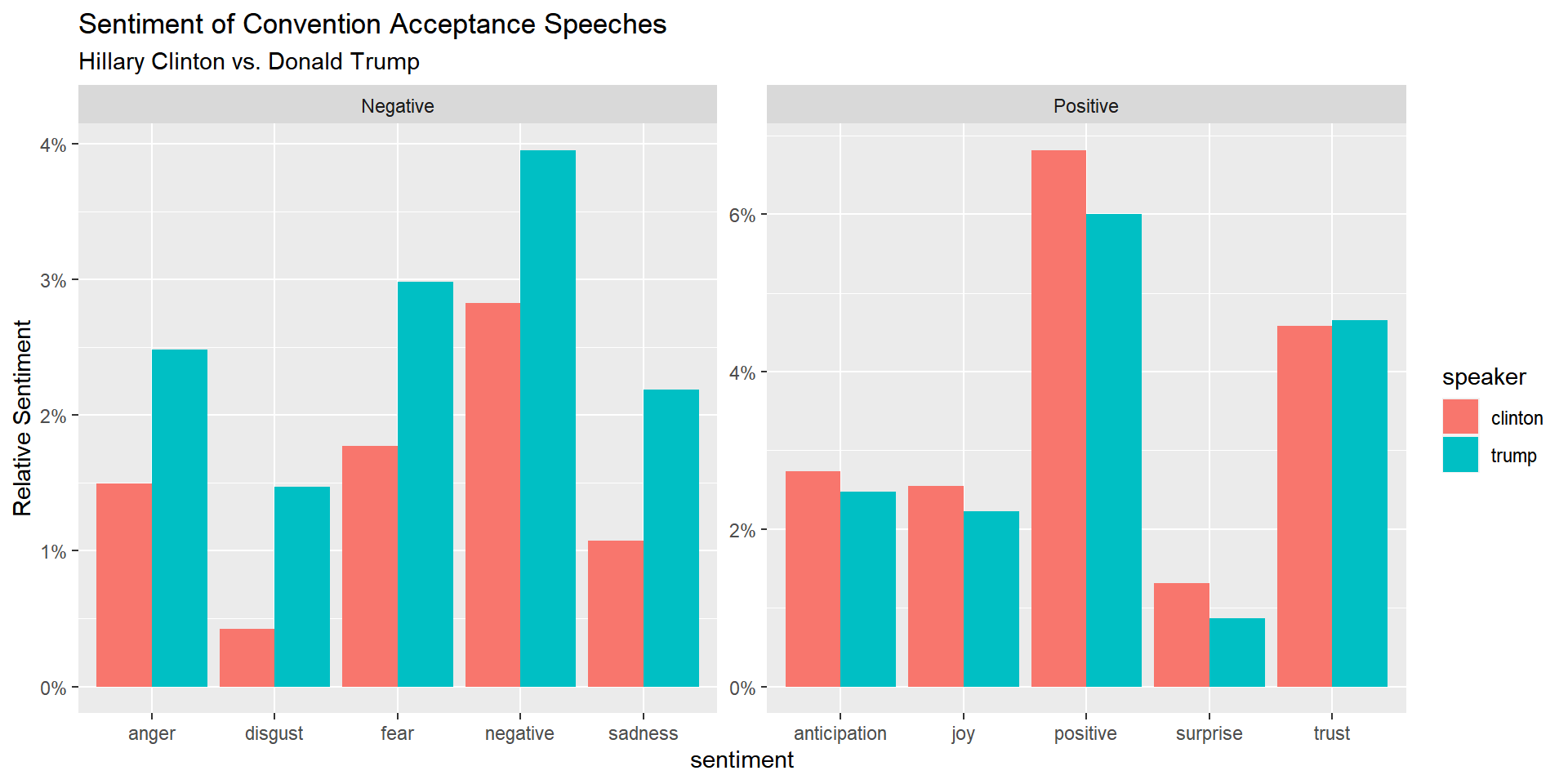
Case Study: Sentiments in Las Vegas
Let’s return to the Las Vegas resort reviews and study how average sentiment vary across resorts. We start by loading the review data, cleaning it up and convert to tidy text:
reviews <- read_csv('data/reviewsTripAll.csv')
meta.data <- reviews %>%
  select(hotel,reviewID,reviewRating)

reviewsTidy <- reviews %>%
  unnest_tokens(word,reviewText) %>%
  count(reviewID,word)
Suppose we were interested in the negative and positive sentiment for each resort and the difference between the two, i.e., the net positive sentiment. To do this, first calculate the total number of terms used for each resort:
term.hotel <- reviewsTidy %>%
  inner_join(meta.data,by='reviewID') %>%
  group_by(hotel) %>%
  summarize(n.hotel=sum(n))
Next we join in the sentiment lexicon, summarize total sentiment for each hotel, normalize by total term count by hotel and finally join in the hotel name and visualize the result:
bing <- get_sentiments("bing")

hotel.sentiment <- reviewsTidy %>%
  inner_join(bing,by=c("word")) %>%
  left_join(meta.data,by='reviewID') %>%
  group_by(hotel,sentiment) %>%
  summarize(total=sum(n)) %>%
  inner_join(term.hotel,by='hotel') %>%
  mutate(relative.sentiment = total/n.hotel)


hotel.sentiment %>%
  ggplot(aes(x=sentiment,y=relative.sentiment,fill=sentiment)) + geom_bar(stat='identity') +
  facet_wrap(~hotel)+ theme(axis.text.x = element_text(angle = 45, hjust = 1))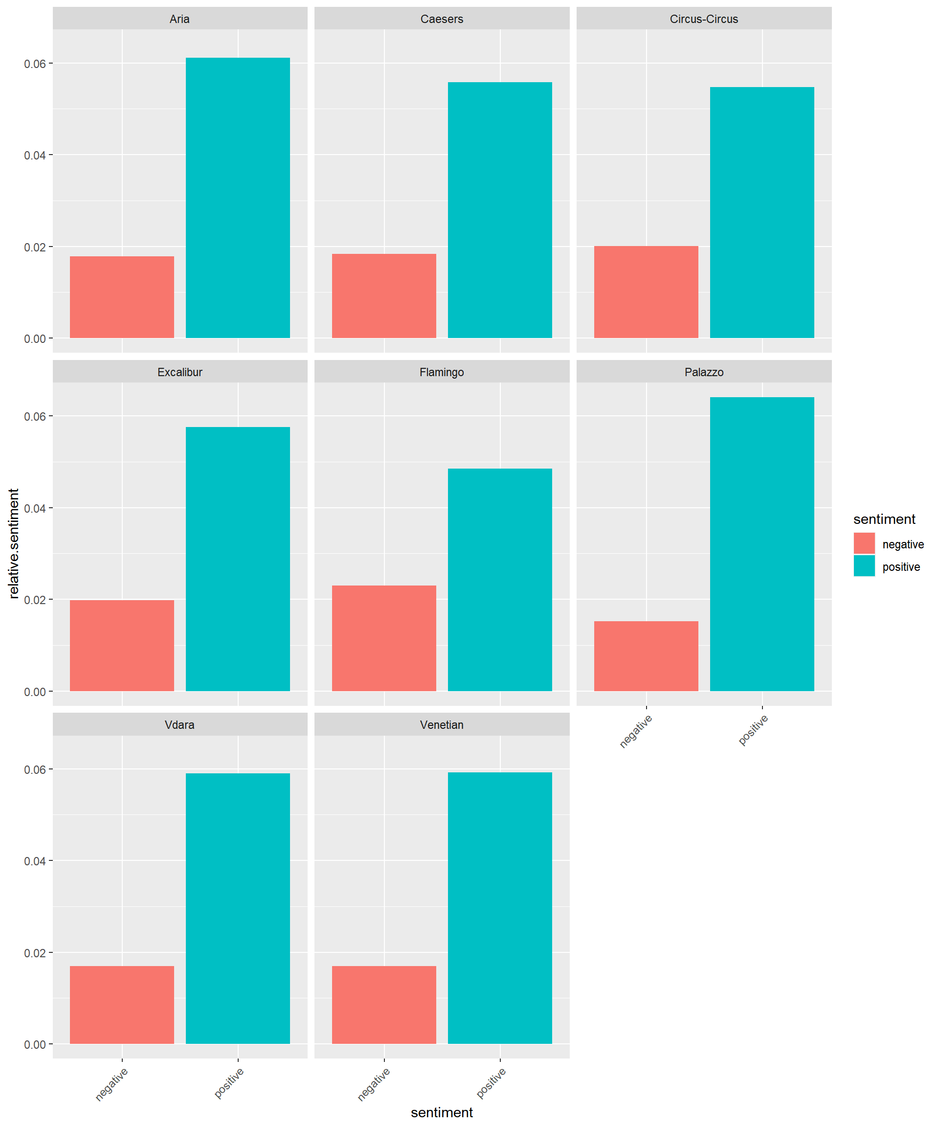
This is a nice visualization but to see the actual net positive sentiment differences across hotels, this one is probably better:
hotel.sentiment %>%
  select(sentiment,relative.sentiment,hotel) %>%
  spread(sentiment,relative.sentiment) %>%
  mutate(net.pos = positive-negative) %>%
  ggplot(aes(x=fct_reorder(hotel,net.pos),y=net.pos)) + geom_point(size=4) + coord_flip()+
  scale_y_continuous(labels=percent)+ylab('Net Positive Sentiment')+xlab('Resort')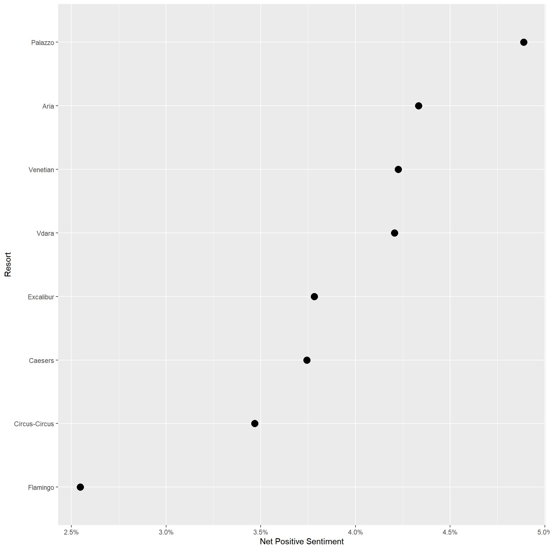
Finally, we can try to look at a wider range of sentiments:
nrc <- get_sentiments("nrc")

hotel.sentiment <- reviewsTidy %>%
  inner_join(nrc,by=c("word")) %>%
  left_join(meta.data,,by='reviewID') %>%
  group_by(hotel,sentiment) %>%
  summarize(total=sum(n)) %>%
  inner_join(term.hotel,by='hotel') %>%
  mutate(relative.sentiment = total/n.hotel)


hotel.sentiment %>%
  ggplot(aes(x=sentiment,y=relative.sentiment,fill=sentiment)) + geom_bar(stat='identity') +
  facet_wrap(~hotel,ncol=3)+ theme(axis.text.x = element_text(angle = 45, hjust = 1)) +
  theme(legend.position="none")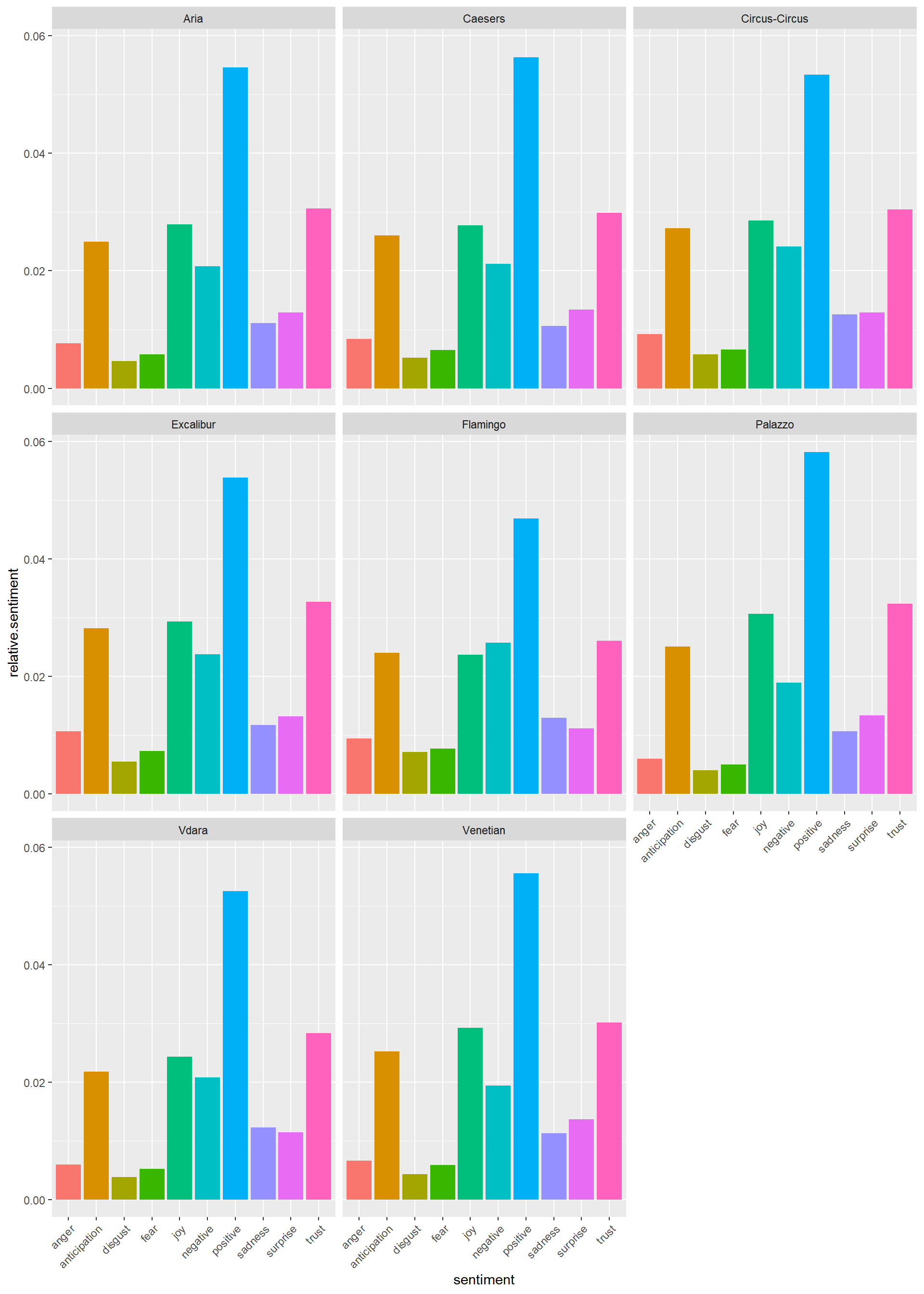
Exercise
If sentiment analysis is worth anything, then positive vs. negative sentiment of a review should be able to predict the star rating. In this exercise you will investigate if this is true.
Using the reviews.tidy and meta.data from above follow the following steps:
- Join the sentiments from the “afinn” lexicon with the reviewsTidy data frame.
- Look at the resulting data frame and make sure you understand the result
- Then for each document calculate the total sentiment score (remember that in the afinn lexicon words are given a score from -5 to 5 where higher is more positive)
- Join the meta.data to the result in 3.
Using your resulting data frame in 4., what can you say about the relationship between sentiments and star rating?
Sentiment Scoring with Python/NLTK
The simple sentiment scoring used above will give a rough approximation to the true underlying sentiments. However, there’s room for improvement. Consider the following text:
example <- read_csv('data/example.csv')
example
Rows: 4 Columns: 2
-- Column specification --------------------------------------------------------
Delimiter: ","
chr (1): text
dbl (1): id
i Use `spec()` to retrieve the full column specification for this data.
i Specify the column types or set `show_col_types = FALSE` to quiet this message.# A tibble: 4 x 2
id text
<dbl> <chr>
1 1 This is a great product - I really love it. I received my order quickly~
2 2 This is a great product - I really love it. I received my order quickly~
3 3 What a horrible product! It's totally useless. There is no point in buy~
4 4 This is not a terrible product. It really isn't that bad. It also not g~For this purpose we can use VADER which is part of the NLTK library. VADER stands for Valence Aware Dictionary for sEntiment Reasoner) and has a model that can deal with problem text like “not great” (ie, negations) and is also sensitive to intensity of language or amplifiers (“very happy” vs “happy”). Let’s load this library:
import nltk
nltk.download("vader_lexicon") # only need to run this once
True
[nltk_data] Downloading package vader_lexicon to
[nltk_data] C:\Users\k4hansen\AppData\Roaming\nltk_data...
[nltk_data] Package vader_lexicon is already up-to-date!from nltk.sentiment.vader import SentimentIntensityAnalyzer
vader = SentimentIntensityAnalyzer()
import pandas as pdTo see how this works consider the following small example:
If we use our approach from above we get:
exampleTidy <- example %>%
   unnest_tokens(word,text)

exampleTidy %>%
  count(id,word) %>%
  inner_join(get_sentiments("bing"),by="word") %>%
  group_by(id,sentiment) %>%
  summarize(total=sum(n)) %>%
  pivot_wider(id_cols = 'id',names_from = 'sentiment', values_from = 'total') %>%
  mutate(net.positve=positive-negative)
`summarise()` has grouped output by 'id'. You can override using the `.groups`
argument.# A tibble: 4 x 4
# Groups: id [4]
id negative positive net.positve
<dbl> <int> <int> <int>
1 1 1 4 3
2 2 1 3 2
3 3 2 1 -1
4 4 2 1 -1According to this, the first document has the highest score which doesn’t make sense since the second document is clearly more positive. It also doesn’t make sense that the third and fourth document has the same score.
Running this example through the VADER model we get
sentiments = [vader.polarity_scores(document) for document in example['text']]
sentiments
[{'neg': 0.21, 'neu': 0.544, 'pos': 0.246, 'compound': 0.2818}, {'neg': 0.167, 'neu': 0.41, 'pos': 0.423, 'compound': 0.8588}, {'neg': 0.342, 'neu': 0.564, 'pos': 0.094, 'compound': -0.7639}, {'neg': 0.165, 'neu': 0.551, 'pos': 0.284, 'compound': 0.3343}]Much better! The function scores each document for positive sentiment, negative sentiment, neutral and then an overall score (“compound”). Positive compound scores signify an overall positive document (and opposite for negative).
Let’s run this on our hotel review data:
reviews = pd.read_csv('data/vegas_hotel_reviews.csv')
business = pd.read_csv('data/vegas_hotel_info.csv')[["business_id", "name"]]
We first get polarity scores on each review:
reviews["scores"] = reviews["text"].apply(lambda text: vader.polarity_scores(text))we then focus on overall sentiment and extract the compound scores:
reviews["compound"] = reviews["scores"].apply(lambda score_dict: score_dict["compound"])To get a quick gut-check that these scores are meaningful, we should expect average polarity scores to increase with the star rating of the review. Let’s check:
scoreByStar = reviews.groupby(['stars'])['compound'].mean().reset_index()
print(scoreByStar)
stars compound
0 1 -0.121242
1 2 0.283465
2 3 0.669230
3 4 0.866542
4 5 0.889663We can also calculate average polarity score for each hotel and use this as an indirect measure of hotel quality. Which hotels come out on top?
scoreByHotel = reviews.groupby(['business_id'])['compound'].mean().reset_index()
scoreByHotel = scoreByHotel.merge(business, on = 'business_id').sort_values(by=['compound'], ascending = False)
print(scoreByHotel)
business_id ... name
0 -7yF42k0CcJhtPw51oaOqQ ... Bellagio
4 AtjsjFzalWqJ7S9DUFQ4bw ... The Cosmopolitan of Las Vegas
1 34uJtlPnKicSaX1V8_tu1A ... The Venetian Resort Hotel Casino
5 DUdBbrvqfaqUe9GYKmYNtA ... The Mirage
7 JpHE7yhMS5ehA9e8WG_ETg ... Aria Hotel & Casino
6 HMr_KN63f6MzM9h8Wije3Q ... New York - New York
16 uJYw4p59AKh8c8h5yWMdOw ... Planet Hollywood Las Vegas Resort & Casino
10 TWD8c5-P7w9v-2KX_GSNZQ ... Mandalay Bay Resort & Casino
11 _v6HIliEOn0l0YaAmBOrxw ... Treasure Island
13 eWPFXL1Bmu1ImtIa2Rqliw ... MGM Grand Hotel
14 kEC7OlpPnZRxCUyVwq7hig ... Hard Rock Hotel & Casino
17 z3SyT8blMIhsZNvKJgKcRA ... Caesars Palace Las Vegas Hotel & Casino
12 bYhpy9u8fKkGhYHtvYXazQ ... Paris Las Vegas Hotel & Casino
15 ripCiWZ0MblMZSLrIKQAKA ... Monte Carlo Hotel And Casino
3 8IMEf_cj8KyTQojhNOyoPg ... Rio All Suites Hotel & Casino
8 NGJDjdiDJHmN2xxU7KauuA ... Flamingo Las Vegas Hotel & Casino
2 6LM_Klmp3hOP0JmsMCKRqQ ... Luxor Hotel And Casino Las Vegas
9 RbkLrCFa2AL1K25GCnNK8A ... LVH - Las Vegas Hotel & Casino
[18 rows x 3 columns]