Predicting Binary Events

In this section we will develop methods for predicting binary events. These are events that either occur or don’t occur. For example, will a certain customer place a new order in the next month? Clearly, this will either happen or not happen. In order to do this we need to modify our approach from the one we used when discussing linear predictive models. These were models of the mean of a continuous variable, e.g., log price. What we need to do now is to model the mean of a binary variable, e.g., a probability. If the predicted probability of the event occurring is high we will predict that it is likely that the event will occur. Since we are modelling probabilities we need to make sure that the predicted probabalities are constrained to be between zero and one. The most popular model for doing this is the Logit Model.

You can download the code and data for this module by using this dropbox link: https://www.dropbox.com/sh/zkkp7ul5gg0jmgb/AADwTkVfZWacgj6doBxokFfpa?dl=0. If you are using Rstudio you can do this from within Rstudio:

usethis::use_course("https://www.dropbox.com/sh/zkkp7ul5gg0jmgb/AADwTkVfZWacgj6doBxokFfpa?dl=1")

Logit Models

Suppose we want to understand what drives some users to click on an online banner ad. In this case we can let \(Y\) denote the binary event with \[ Y_i= \begin{cases} 1 & \text{if user i clicks on the ad,} \\ 0 & \text{otherwise.} \end{cases} \] Suppose the online advertiser randomly changes the image shown on the add from the standard image \(X=0\) to a new test image \(X=1\). We want to predict by how the test image changes the click-rate. Suppose we have data \((Y_i,X_i)\) from a large set of users. Some users were exposed to the standard image while others were exposed to the new image. A logit model will model the click rate as \[ {\rm Pr}(Y_i=1|X_i) = \frac{\exp\lbrace \beta_0 + \beta_X X_i \rbrace }{1 + \exp\lbrace \beta_0 + \beta_X X_i \rbrace}, \] where \(\beta_0\) and \(\beta_X\) are unknown parameters to be determined by the historical data. Let’s make some quick observations. First, this model constrains the predicted probabilities to be between zero and one. Second, we can use this model to see what the change in click-rate will be when we change the image. This is easy - just plug in: \[ {\rm Pr}(\text{click}|\text{standard image}) = {\rm Pr}(Y_i=1|X_i=0) = \frac{\exp\lbrace \beta_0 \rbrace }{1 + \exp\lbrace \beta_0 \rbrace}. \] Using the historical data (and the power of R!) we can determine \(\beta_0\) - we will see how to do this below. Similarly, \[ {\rm Pr}(\text{click}|\text{new image}) = {\rm Pr}(Y_i=1|X_i=1) = \frac{\exp\lbrace \beta_0 + \beta_X \rbrace }{1 + \exp\lbrace \beta_0 + \beta_X \rbrace}. \] Therefore we get \[ \Delta(\text{click rate}) \equiv \frac{\exp\lbrace \beta_0 + \beta_X \rbrace }{1.0 + \exp\lbrace \beta_0 + \beta_X \rbrace} - \frac{\exp\lbrace \beta_0 \rbrace }{1 + \exp\lbrace \beta_0 \rbrace}. \]

Calibrating Logit Models on Data

The standard method used to calibrate the \(\beta\) weights of a logit model is Maximum Likelihood. This is based on choosing \(\beta\) to maximize the total probability of the training data. Suppose the training data is \(\lbrace Y_i,X_i \rbrace_{i=1}^N\) where \(X_i\) are the \(K\) predictor variables for person \(i\). Define \[ \mu_i \equiv \sum_{k=1}^K \beta_k X_{ik}. \] The probability of observing \(Y_i\) depends on what \(Y_i\) is - 1 or 0: \[ \begin{align*} {\rm Pr}(Y_i=1|X_i) & = \frac{\exp\lbrace \mu_i \rbrace }{1.0 + \exp\lbrace \mu_i\rbrace}, \\ {\rm Pr}(Y_i=0|X_i) & = \frac{1 }{1 + \exp\lbrace \mu_i\rbrace}. \end{align*} \] Therefore we can write the probability of observing \(Y_i\) as \[ L_i(\beta) \equiv \left(\frac{\exp\lbrace \mu_i \rbrace }{1.0 + \exp\lbrace \mu_i\rbrace} \right) ^{Y_i} \times \left(\frac{1 }{1 + \exp\lbrace \mu_i\rbrace} \right) ^{1-Y_i} \] If - in addition - we assume that \(Y_i\) is generated independently of all other \(Y_i\)’s, then we can write the probability of observing the full training sample as \[ L(\beta) = \prod_{i=1}^N L_i(\beta). \] The method of Maximum Likelihood uses a numerical algorithm to find the \(\beta\) that maximizes \(L(\beta)\). Technically, since it turns out to be easier to maximize the log of \(L\), it will maximize \(\log L(\beta)\).

Case Study: Titanic

You are about to board the Titanic - would you rather be Jack or Rose? Well, of course we know what happened in the movie - but was this representative of the actual survival rates of rich young women vs. poor young men? And what about old men or women? Let’s build a logit model to predict survival probabilities for different traveller segments on the Titanic.

First, we need the actual passenger data for Titanic with information on demographics and survival outcomes. It turns out that this exists - although it is incomplete: We only have survival information on 1309 of the more than 2000 passengers and complete demographics only for 1046 passengers. However, let’s see what we can do with what we have. First, load the data and see what variables we have:

## load libraries
library(tidyverse)
library(glmnet)

## get the data 
train <- read_csv('data/titanic_train.csv')
validation <- read_csv('data/titanic_validation.csv')

## what's in the data?
head(train)

# A tibble: 6 x 15
     id pclass survived name         sex     age sibsp parch  ticket  fare cabin
  <dbl> <chr>  <chr>    <chr>        <chr> <dbl> <dbl> <dbl>   <dbl> <dbl> <chr>
1   472 2nd    Yes      "Kelly, Mrs~ fema~    45     0     0  223596 13.5  <NA> 
2   370 2nd    No       "Chapman, M~ fema~    29     1     0      NA 26    <NA> 
3   889 3rd    No       "Johanson, ~ male     34     0     0 3101264  6.50 <NA> 
4   628 3rd    No       "Andersson,~ fema~     9     4     2  347082 31.3  <NA> 
5   319 1st    No       "Williams-L~ male     NA     0     0  113510 35    C128 
6  1115 3rd    No       "Pearce, Mr~ male     NA     0     0  343271  7    <NA> 
# i 4 more variables: embarked <chr>, boat <chr>, body <dbl>, home.dest <chr>

Ok - looks like we have class of travel, survival outcome, name, gender, age. There is also information on number of siblings/spouses aboard (sibsp) and number of parents/childen aboard (parch). You can also see ticket number and price, cabin number, where the traveller embarked and home destination. For survivors you can see which lifeboard they were on and for non-survivors you can see whether the body was recovered. The data has been split into 1047 passengers in the training sample and 262 in the validation sample.

To see what might matter for survival, let’s quickly make some bar charts focusing on class of travel, age and gender:

## by class of travel
train %>%
  ggplot(aes(x=pclass,fill=survived)) + geom_bar(position='dodge') + xlab('Class of Travel')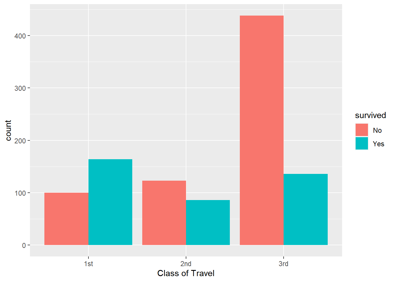

## by gender
train %>%
  ggplot(aes(x=sex,fill=survived)) + geom_bar(position='dodge')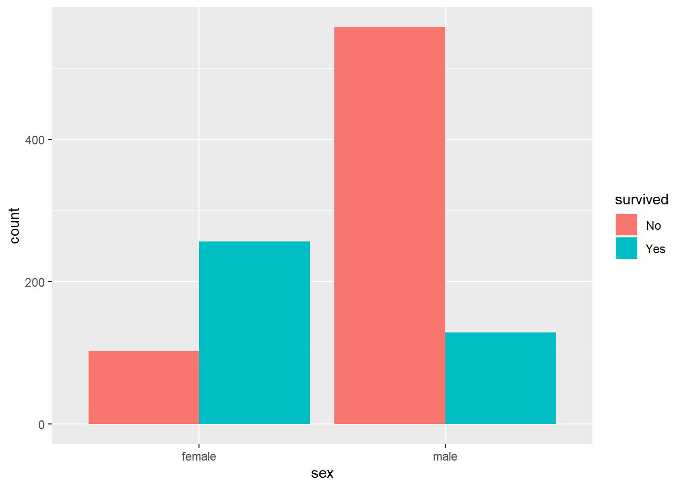 

## by age
train %>%
  filter(!age=='NA') %>%
  mutate(age.f=cut(age,breaks=c(0,20,30,40,50,60,100))) %>%
  ggplot(aes(x=age.f,fill=survived)) + geom_bar(position='dodge') + xlab('Age Group')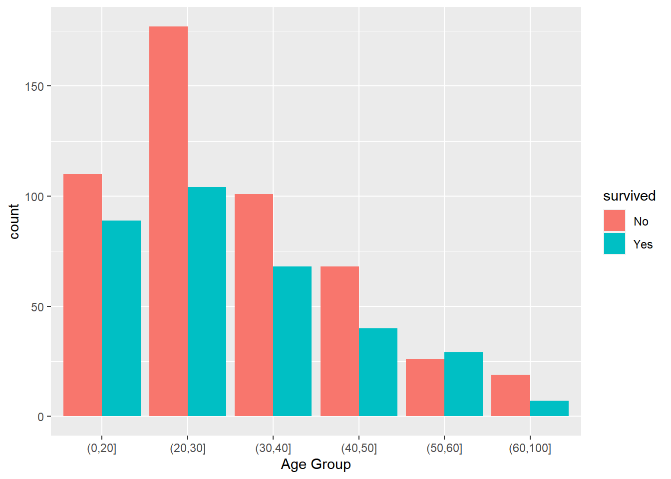

Hmm…it’s pretty clear that passengers travelling on 3rd class didn’t fare well compared to 1st and 2nd class passengers, and 2nd class passengers were worse off compared to 1st class. We also see a huge gender effect - many more female passengers survived. It is a bit harder to judge the age effect. However, it seems like the survival rate is much lower for 20-30 year olds than any of the other categories.

Python

There are several Python libraries available for training logit classifiers. Here we will use scikit-learn. We load the required libraries and the data. Furthermore, knowing what we know from above, we also drop passengers with missing age information:

import pandas as pd
import numpy as np
from sklearn.linear_model import LogisticRegression
from sklearn.metrics import classification_report, confusion_matrix

## get titanic.data ---------------------------------------------------------
train = pd.read_csv('data/titanic_train.csv')
validation = pd.read_csv('data/titanic_validation.csv')
train = train.dropna(subset=['age'])
validation = validation.dropna(subset=['age'])

allDF = pd.concat([train, validation])
nTrain = train.shape[0]
nAll = allDF.shape[0]

Next we define age bins like above and create the feature matrix using the get_dummies function from pandas for both the training and validation data:

allDF['age_f'] = pd.cut(allDF["age"],bins=[0,20,30,40,50,100])

Xdf = allDF[['pclass','sex','age_f']].copy()
X = pd.get_dummies(data=Xdf, drop_first=True)
y = allDF['survived']

X_train = X[0:nTrain]
y_train = y[0:nTrain]
X_valid = X[nTrain:nAll]
y_valid = y[nTrain:nAll]

Now we are ready to train our classifier. We initialize a LogisticRegression object and specify that we wish to train the model without any penalty/regularization term (the default is an L2 penalty so we need to override this). We then train the model using only the training data:

model = LogisticRegression(penalty = "none")
model.fit(X_train, y_train)

LogisticRegression(penalty='none')

In a Jupyter environment, please rerun this cell to show the HTML representation or trust the notebook.
On GitHub, the HTML representation is unable to render, please try loading this page with nbviewer.org.

We can inspect the trained weights for the classifier:

# weights
model.intercept_

array([2.89516993])

model.coef_

array([[-1.22938318, -2.25319286, -2.44926147, -0.39705775, -0.47139706,
        -1.14135252, -1.14302393]])

This is identical to what we got in the R version. Next, we can predict on the validation data and summarize the performance:

## predictions on validation
y_pred = model.predict(X_valid)
y_pred_prob = model.predict_proba(X_valid)

## confusion matrix 
cm = confusion_matrix(y_valid, y_pred)
print(cm)

[[98 20]
 [24 66]]

cr = classification_report(y_valid, y_pred)
print(cr)

              precision    recall  f1-score   support

          No       0.80      0.83      0.82       118
         Yes       0.77      0.73      0.75        90

    accuracy                           0.79       208
   macro avg       0.79      0.78      0.78       208
weighted avg       0.79      0.79      0.79       208

The confusion matrix is identical to the one we got using R. Here we have also calculated a set of additional performance metrics using the classification_report function. These metrics are useful when more detailed insights into the model’s performance is needed. Precision is the fraction of predicted positives (here survivals) that are correct while recall is the fraction of actual positives that the model predicts correctly. These metrics can be relevant when prediction errors have differential costs to the decision maker. For example, if false positives (an actual dead person is predicted to have survived) are very costly, then precision should be monitored. On the hand, if false negatives (an actual survivor is predicted to have died) are more costly, then recall is important. The F1 score is a balance of these two considerations as is defined as 2(precisionrecall)/(precision + recall).

Finally, let’s add the same interaction we did in the R version: class of travel interacted with gender:

X = pd.get_dummies(data=Xdf, drop_first=True)
X['pclass_2nd:male'] = X['pclass_2nd']*X['sex_male']
X['pclass_3rd:male'] = X['pclass_3rd']*X['sex_male']

X_train = X[0:nTrain]
X_valid = X[nTrain:nAll]

Let’s train this model on the training data and inspect the trained weights:

model = LogisticRegression(penalty = "none")
model.fit(X_train, y_train)

# weights

LogisticRegression(penalty='none')

In a Jupyter environment, please rerun this cell to show the HTML representation or trust the notebook.
On GitHub, the HTML representation is unable to render, please try loading this page with nbviewer.org.

print(model.intercept_)

[4.41031257]

print(model.coef_)

[[-2.06175908 -4.25064979 -4.19472317 -0.44791979 -0.50366059 -1.20807825
  -1.28639893  0.74460798  2.73386649]]

Again - same results as in the R version. Finally, we form predictions on the validation data:

## predictions on validation
y_pred = model.predict(X_valid)
y_pred_prob = model.predict_proba(X_valid)

## confusion matrix 
cm = confusion_matrix(y_valid, y_pred)
print(cm)

[[111   7]
 [ 33  57]]

cr = classification_report(y_valid, y_pred)
print(cr)

              precision    recall  f1-score   support

          No       0.77      0.94      0.85       118
         Yes       0.89      0.63      0.74        90

    accuracy                           0.81       208
   macro avg       0.83      0.79      0.79       208
weighted avg       0.82      0.81      0.80       208

The second model has higher accuracy. It achieves this by being better at predicting non-survival compared to Model A. Note that Model B is slightly worse than A at predicting survival.

R

Based on these summaries, it seems reasonable to try out a logit model with class of travel, gender and age as predictor variables. The syntax for setting up a logit model is more or less the same as the one we used for linear predictive models:

## remove observations with missing age, define age groups and survival outcome
train <- train %>%
  filter(!age=='NA') %>%
  mutate(age.f=cut(age,breaks=c(0,20,30,40,50,100)),
         lsurv = survived=='Yes',
         pclass = factor(pclass),
         sex = factor(sex))
     
validation <- validation %>%
  filter(!age=='NA') %>%
  mutate(age.f=cut(age,breaks=c(0,20,30,40,50,100)),
         lsurv = survived=='Yes',
         pclass = factor(pclass),
         sex = factor(sex))

## define logit model: class of travel, gender, age group ----------------------
logitTitanicA <- glm(lsurv~pclass+sex+age.f,
                       data=train,
                       family=binomial(link="logit"))

This sets up a logit model for predicting the event that survived is equal to Yes. You can see the individual effects by looking at the results:

summary(logitTitanicA)

Call:
glm(formula = lsurv ~ pclass + sex + age.f, family = binomial(link = "logit"), 
    data = train)

Deviance Residuals: 
    Min       1Q   Median       3Q      Max  
-2.2703  -0.7083  -0.4575   0.6751   2.4494  

Coefficients:
              Estimate Std. Error z value Pr(>|z|)    
(Intercept)     2.8952     0.3043   9.514  < 2e-16 ***
pclass2nd      -1.2294     0.2527  -4.866 1.14e-06 ***
pclass3rd      -2.2532     0.2484  -9.070  < 2e-16 ***
sexmale        -2.4493     0.1858 -13.186  < 2e-16 ***
age.f(20,30]   -0.3971     0.2401  -1.654 0.098131 .  
age.f(30,40]   -0.4714     0.2777  -1.698 0.089568 .  
age.f(40,50]   -1.1414     0.3273  -3.487 0.000488 ***
age.f(50,100]  -1.1430     0.3703  -3.087 0.002024 ** 
---
Signif. codes:  0 '***' 0.001 '**' 0.01 '*' 0.05 '.' 0.1 ' ' 1

(Dispersion parameter for binomial family taken to be 1)

    Null deviance: 1129.41  on 837  degrees of freedom
Residual deviance:  792.11  on 830  degrees of freedom
AIC: 808.11

Number of Fisher Scoring iterations: 4

In a moment we will use R to automatically generate preditions for different traveller segments, but before we do that it might be instructive to see how to do this manually. Suppose we wanted the predicted survival probability for 25 year old males, travelling on 3rd class. We can piece together the \(\beta\) effects for this segment by simply picking out the relevant ones from the table above - remembering to always include the intercept: \[ 2.8952 - 2.2532 - 2.4493 - 0.3971 \approx -2.20 \] Then - applying the logit formula - we get a predicted survival rate of \[ {\rm Pr}(\text{survival}| \text{25 year, 3rd class, male} ) = \exp(-2.20)/(1.0 + \exp(-2.20)) \approx 10\% \] Those are bad odds - only 1 in 10 survived. Let’s calculate this for all segments. To do this we create a new data frame where each row is a segment for which we want a predicted survival rate:

## create prediction array 
predDF <- expand.grid(pclass=levels(train$pclass), 
                       sex=levels(train$sex),
                       age.f=levels(train$age.f))

## make predictions
predDF$Prob <- predict(logitTitanicA, 
                        newdata = predDF, 
                        type = "response")

The data frame predDF contains all possible combinations of our three predictor variables. Sometimes - when you have many predictor variables - you might not be interested in all combinations and you would only use a subset of all possibilities. Here we will use all of them (30 in total). The second command use the logit model to predict the probability (“response”) for each of the rows in predDF.

Let’s check that our manual calculation above was correct:

predDF %>% 
  filter(sex=='male', pclass=='3rd')

  pclass  sex    age.f       Prob
1    3rd male   (0,20] 0.14096462
2    3rd male  (20,30] 0.09935783
3    3rd male  (30,40] 0.09290324
4    3rd male  (40,50] 0.04979937
5    3rd male (50,100] 0.04972038

These are the predicted survival rates for males travelling on 3rd class. We can see that we got it right above.

At this point it might be fun to visualize the predictions for all segments:

## plot predictions
predDF %>%
  ggplot(aes(x=age.f,y=Prob,group=sex,color=sex)) + geom_line(linetype='dotted') + 
  geom_point() + 
  ylab('Survival Probability') + xlab('Age Group') + 
  facet_wrap(~pclass) + 
  theme(axis.text.x = element_text(angle = 45, hjust = 1),
        plot.title=element_text(size=14))+
  ggtitle('Predicted Survival Probability by Class of Travel, Gender and Age')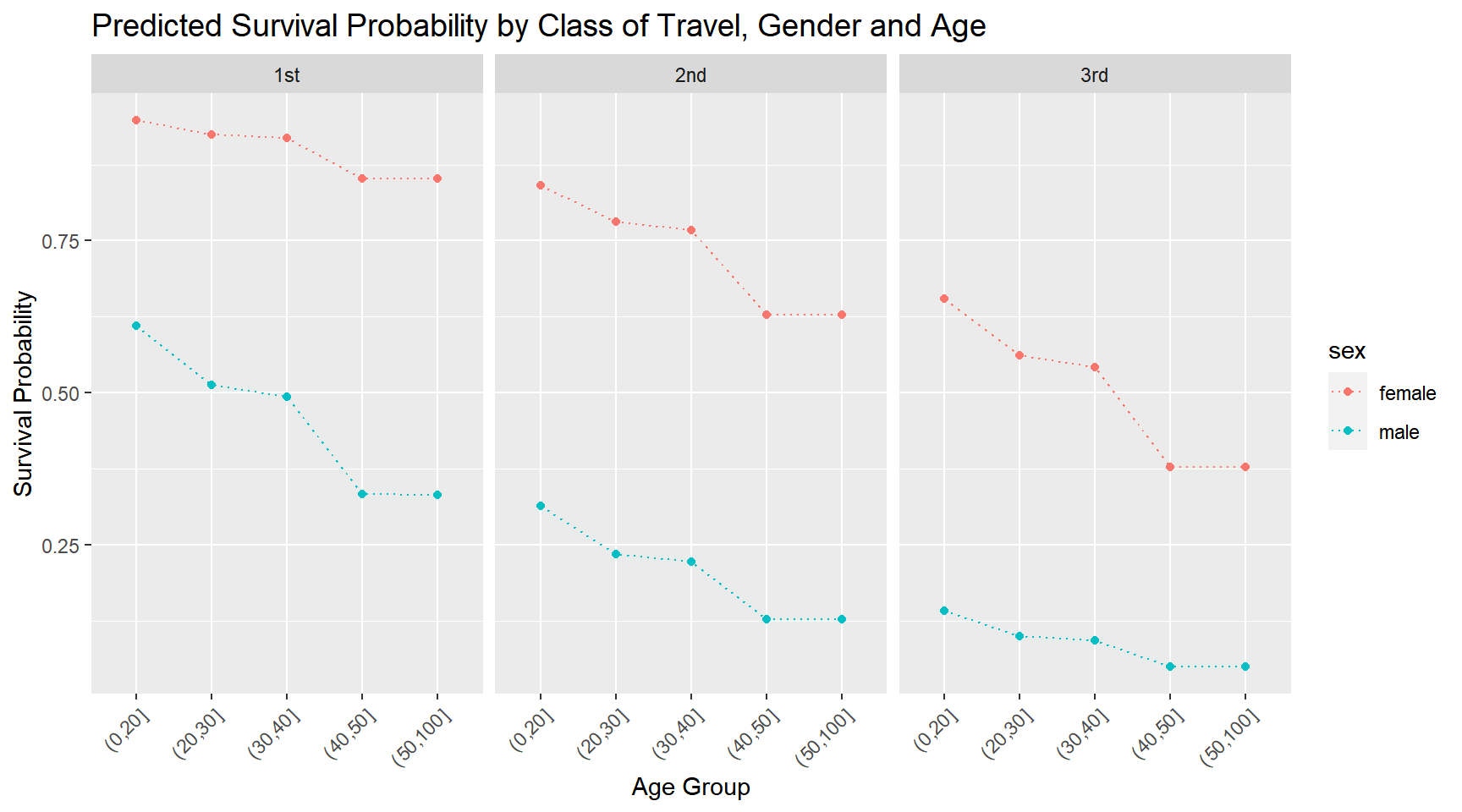

What would you conclude about demographics and survival rates based on this?

Is the model above reasonable? Maybe - but one objection we could raise is the way we have modelled the impact of gender and class of travel. Notice that by design, the effect of gender is the same for every class of travel. This is a consequence of the additivity assumption implicit in the model above. Specifically, the difference in the sum of \(\beta\)’s for males and females on 1st class is identical to the difference in the sum of \(\beta\)’s for males and females on 3rd class. We can change this by adding an interaction in the model:

logitTitanicB <- glm((survived=='Yes')~pclass*sex+age.f,
                       data=train,
                       family=binomial(link="logit"))

summary(logitTitanicB)

Call:
glm(formula = (survived == "Yes") ~ pclass * sex + age.f, family = binomial(link = "logit"), 
    data = train)

Deviance Residuals: 
    Min       1Q   Median       3Q      Max  
-2.8218  -0.6939  -0.5519   0.5027   2.2748  

Coefficients:
                  Estimate Std. Error z value Pr(>|z|)    
(Intercept)         4.4107     0.6350   6.946 3.75e-12 ***
pclass2nd          -2.0623     0.6902  -2.988 0.002809 ** 
pclass3rd          -4.2510     0.6375  -6.668 2.59e-11 ***
sexmale            -4.1950     0.6192  -6.774 1.25e-11 ***
age.f(20,30]       -0.4481     0.2346  -1.910 0.056086 .  
age.f(30,40]       -0.5038     0.2764  -1.823 0.068309 .  
age.f(40,50]       -1.2082     0.3475  -3.477 0.000507 ***
age.f(50,100]      -1.2865     0.4129  -3.116 0.001832 ** 
pclass2nd:sexmale   0.7453     0.7503   0.993 0.320571    
pclass3rd:sexmale   2.7342     0.6665   4.102 4.09e-05 ***
---
Signif. codes:  0 '***' 0.001 '**' 0.01 '*' 0.05 '.' 0.1 ' ' 1

(Dispersion parameter for binomial family taken to be 1)

    Null deviance: 1129.41  on 837  degrees of freedom
Residual deviance:  758.17  on 828  degrees of freedom
AIC: 778.17

Number of Fisher Scoring iterations: 6

The gender effect now depends on class of travel: In 1st class, the gender effect for males and females is -4.19. For 3rd class it is -4.19+2.73 = -1.46. What does this mean? It means that the relative difference in survival rates for males and females is much bigger in 1st class than 3rd class. We can see this better by visualizing the implied survival rates:

predDF$Prob <- predict(logitTitanicB, 
                        newdata = predDF, 
                        type = "response")

predDF %>%
  ggplot(aes(x=age.f,y=Prob,group=sex,color=sex)) + geom_line(linetype='dotted') + 
  geom_point() + 
  ylab('Survival Probability') + xlab('Age Group') + 
  facet_wrap(~pclass) + 
  theme(axis.text.x = element_text(angle = 45, hjust = 1),
        plot.title=element_text(size=14))+
  ggtitle('Predicted Survival Probability by Class of Travel, Gender and Age')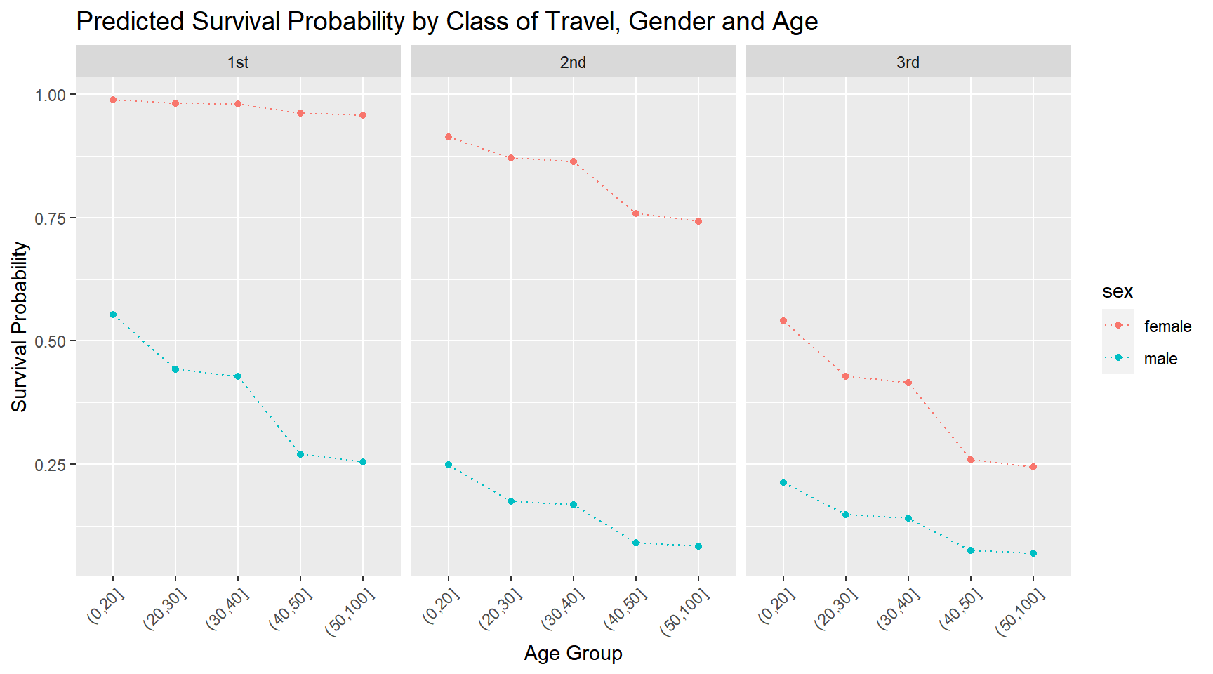

Compare this to the previous plot.

One thing we haven’t done is to see how well our model actually predicts survival rates for the “validation” passengers. We can use the predict function on the test data to do this:

validation <- validation %>%
  mutate(ProbRepA = predict(logitTitanicA,newdata = validation,type = "response"),
         ProbRepB = predict(logitTitanicB,newdata = validation,type = "response"),
         SurvPredA = ProbRepA > 0.5,
         SurvPredB = ProbRepB > 0.5)

We first get the predicted survival probabilities for each validation passenger and then use them to predict survival if the probability is above 50% (otherwise no survival is predicted). We can now tally up our predictions and see how we did. This is usefully presented in a table called a confusion matrix. This table simply counts how many times we got a prediction right or wrong:

TabPredA <- table(validation$lsurv,validation$SurvPredA)
TabPredB <- table(validation$lsurv,validation$SurvPredB)

Let’s look at the first table:

TabPredA

       
        FALSE TRUE
  FALSE    98   20
  TRUE     24   66

Remember that “TRUE” means survival. There were a total of 90 validation passengers who survived. This is the sum of the second row in the table. The columns indicate our predictions of the fate of these passengers. Model A correctly predicted that 66 of these 90 passengers survived. It wrongly predicted that 24 of them died. Similarly - looking at the first row - there were a total of 118 validation passengers who died. We correcly predict 98 of these deaths. We can think of the diagonal of the table - normalized by the total - as the overall accuracy of the model. This is

AccuracyA <- (TabPredA[1,1]+TabPredA[2,2])/sum(TabPredA)
AccuracyA

[1] 0.7884615

Let’s compare this to the second model:

AccuracyB <- (TabPredB[1,1]+TabPredB[2,2])/sum(TabPredB)

TabPredB

       
        FALSE TRUE
  FALSE   111    7
  TRUE     33   57

AccuracyB

[1] 0.8076923

The second model has higher accuracy. It achieves this by being better at predicting non-survival compared to Model A. Note that Model B is slightly worse than A at predicting survival.

Case Study: Donors Choose

Let’s return to the DonorsChoose data. The objective is to try to predict which projects gets funded. Here we are using a subset of the full data. There are 60,000 projects in the training data and we will use this data to predict funding success of the 40,000 projects in the test data.

Python

Let’s read in the data and apply a few transformations to get discretize the numerical features:

import pandas as pd
import numpy as np
from sklearn.linear_model import LogisticRegression
from sklearn.metrics import classification_report, confusion_matrix
import datetime

## import  ---------------------------------------------------------
train = pd.read_csv('data/projects_train.csv')
validation = pd.read_csv('data/projects_validation.csv')

allDF = pd.concat([train, validation])
nTrain = train.shape[0]
nAll = allDF.shape[0]

# discretize numeric features
allDF['month'] = pd.Categorical(pd.to_datetime(allDF['date_posted']).dt.month)
allDF['cost'] = pd.cut(allDF["total_price_excluding_optional_support"],
                       bins=[0,200,300,400,500,600,700,800,900,1000,1500,2000,500000])
allDF['nStudents'] = pd.cut(allDF["students_reached"],bins=[0,10,20,30,50,100,200,10000])

# set up feature matrix and target
features = ['primary_focus_subject','grade_level','poverty_level','resource_type',
            'eligible_double_your_impact_match','cost','nStudents',
            'eligible_almost_home_match','month','teacher_teach_for_america',
            'teacher_prefix','school_charter','school_magnet','school_state']

Xdf = allDF[features].copy()

X = pd.get_dummies(data=Xdf, drop_first=True)

y = allDF['funding_status']
X_train = X[0:nTrain]
y_train = y[0:nTrain]
X_valid = X[nTrain:nAll]
y_valid = y[nTrain:nAll]

Ok - let’s train the model on the training data and predict validation success of validation projects:

model = LogisticRegression(penalty = "none",max_iter=1000)
model.fit(X_train, y_train)

## predictions on validation

LogisticRegression(max_iter=1000, penalty='none')

In a Jupyter environment, please rerun this cell to show the HTML representation or trust the notebook.
On GitHub, the HTML representation is unable to render, please try loading this page with nbviewer.org.

y_pred = model.predict(X_valid)
y_pred_prob = model.predict_proba(X_valid)

## confusion matrix 
cm = confusion_matrix(y_valid, y_pred)
print(cm)

[[13274  6797]
 [ 6290 13639]]

cr = classification_report(y_valid, y_pred)
print(cr)

              precision    recall  f1-score   support

   completed       0.68      0.66      0.67     20071
     expired       0.67      0.68      0.68     19929

    accuracy                           0.67     40000
   macro avg       0.67      0.67      0.67     40000
weighted avg       0.67      0.67      0.67     40000

We get an accuracy of 67%. Can you build a logit classifier that will beat this threshold? Try it out!

R

Let’s read in the data and apply a few transformations to get discretize the numerical features:

library(tidyverse)
library(broom)
library(forcats)
library(lubridate)

## get data 

projectsTrain <- read_csv('data/projects_train.csv')
projectsVal <- read_csv('data/projects_validation.csv')

projectsTrain <- projectsTrain %>%
  mutate(cost.group = cut(total_price_excluding_optional_support, 
                          breaks = c(0,200,300,400,500,600,700,800,900,1000,1500,2000,500000)),
         month = as.character(month(date_posted,label = T)),
         nStudents = cut(students_reached,
                         breaks=c(0,10,20,30,50,100,200,10000),
                         include.lowest = T))

projectsVal <- projectsVal %>%
  mutate(cost.group = cut(total_price_excluding_optional_support, 
                          breaks = c(0,200,300,400,500,600,700,800,900,1000,1500,2000,500000)),
         month = as.character(month(date_posted,label = T)),
         nStudents = cut(students_reached,
                         breaks=c(0,10,20,30,50,100,200,10000),
                         include.lowest = T))

Next, we specify a logit model including the main characteristics of each project:

logitProjects <- glm(funding_status=='completed'~
                       primary_focus_subject +
                       grade_level + 
                       poverty_level + 
                       resource_type + 
                       eligible_double_your_impact_match + 
                       cost.group + 
                       nStudents + 
                       eligible_almost_home_match + 
                       month + 
                       teacher_teach_for_america + 
                       teacher_prefix + 
                       school_charter +
                       school_magnet + 
                       school_state,
                     data=projectsTrain,
                     family=binomial(link="logit"))

logitProjectsStats <- tidy(logitProjects)

Let’s see how well we predict the validation projects:

logitProjectsStats <- tidy(logitProjects)

projectsVal$ProbCompleteLogit=predict(logitProjects,newdata = projectsVal,type = "response")
projectsVal$PredStatusLogit=if_else(projectsVal$ProbCompleteLogit > 0.5,'Pred.completed','Pred.expired')

confMat1 <- table(projectsVal$funding_status,projectsVal$PredStatusLogit)
prec1 <- sum(diag(confMat1))/sum(confMat1)

prec1

[1] 0.672725

Can you build a logit classifier that will beat this threshold? Try it out!

Torching Your Logits!

The built-in functions in R (glm) and in the scikit-learn library are easy to use and you can train a logit with very little work by using them. However, the algorithms they use don’t scale well to really big datasets (where either the number of cases or the number of features (or both) are large). In this case you might want to code up your logit classifier from scratch using the Torch library. This is available both in R and Python (the latter called PyTorch). There are actually several reasons why you might want to invest some time in learning this library. One is as mentioned - by having algorithms which scale much better to large data contexts - Torch will empower you to train logit classifiers on data of essentially any size. The second reason is that Torch is the de facto state-of-the-art library for training much more advanced predictive models such as deep neural nets.

While Torch was developed to train deep neural networks, it can be used for simpler models too. In fact, a logit classifier can be expressed as a one-layer neural network. In the following we will take advantage of this and show how we can train a logit classifier on a very large dataset using Torch.

Python

Let’s try setting up a logit classifier in Torch. We will use some synthetic data: 200,000 cases with 100 features. This is a fairly large scale classifaction task. We start by importing the relevant libraries and import the data. Also PyTorch requires us to convert dataframes to numpy arrays so we do that immediately:

import torch
import pandas as pd 
import numpy as np
from torch.utils.data import Dataset, DataLoader

## read data 
theFile = "data/logitData.csv"
rawData = pd.read_csv(theFile).to_numpy()
nFull = rawData.shape[0]
input_dim = 50             # feature dimension

Torch requires that we define classes for the data and for the model we wish to train. Think of classes as a combination of both data and methods (functions). First we set up a class for our data:

# define class for data
class LogitDataset(Dataset):
    def __init__(self):
        # Initialize data
        self.y = torch.from_numpy(rawData[:,0])     # outputs
        self.x = torch.from_numpy(rawData[:,1:])    # inputs/features

    # indexing such that dataset[i] can be used to get i-th sample
    def __getitem__(self, index):
        return self.x[index], self.y[index]

    # we can call len(dataset) to return the size
    def __len__(self):
        return len(self.y)

Ok - what is going on here? The LogitDataset class defines a class which inherits the properties of the abstract Torch Dataset class. The abstract Dataset class has two methods that you ALWAYS need to override when you create your own class: getitem returns a single item (or row) of the data - split into input features and output. This is needed for the dataLoader which we will set up below. The method len just returns the number of cases. To initialize a dataset we simly take the full data and convert it to Torch tensors (Torch models are constructed from Torch tensors - just like of them like arrays - kind of).

Next up we need to define our logit classifier. Models in Torch are versions of Torch modules. A Torch module consist of a series of layers and also a forward function that specifies how the layers and the data are combined to create predictions. A “forward pass” simply means creating predictions using the model. In deep neural nets you will have many layers. We don’t need that here since our model is a shallow one: A logit classifier is simply a neural net with one input layer and one output layer. The input layer is just a linear function of the features where each feature receives a weight that we will calibrate using the training data. We then take this layer and convert using the sigmoid function which defines a logit (i.e., \(f(x) = 1/(1+\exp(-x))\)):

## set up class for logit classifier 
class LogisticRegression(torch.nn.Module):
     def __init__(self, input_dim):
        super(LogisticRegression, self).__init__()
        self.linear = torch.nn.Linear(input_dim, 1)  # sets up a linear layer
     def forward(self, x):        
        m = torch.nn.Sigmoid()                  
        y_pred = m(self.linear(x)).squeeze(1)         # defines logit output layer  
        return y_pred

So all this class does is the following: It defines a linear function of the features \(a + b'X\) and then also provides a method for converting weights \((a,b)\) and features \(X\) to predictions (by simply calculating \(\text{sigmoid}(a+b'X)\)).

Ok - let’s set up the data correctly. First, we will usually want to split the full data into training and validation. Torch has functions built-in that does this automatically:

fullDataTorch = LogitDataset()
train_size = int(0.8 * nFull)    # create 80-20 split
valid_size = nFull - train_size
train_dataset, valid_dataset = torch.utils.data.random_split(fullDataTorch, [train_size, valid_size])

One of the advantages of Torch is that it has implementations of various stochastic gradient descent algorithms. Gradient descent algorithms are simple rules for solving an optimization problem in sequential steps. Suppose we want to minimize a function \(H(x)\), i.e., we want to find the value of \(x\), \(x^*\), that minimizes \(H\). Suppose we start at some point \(x_0\). A gradient descent algorithm then moves to a new point \(x_1\) as \[ x_1 = x_0 - \lambda g(x_0), \] where \(g(x)\) is the gradient of \(H\), i.e., \(g(x) \equiv \partial H(x)/\partial x\) and \(\lambda\) is called the learning rate - some positive fixed number that determines the step size.

If the gradient for the full sample is easily calculated we can simply iterate on this rule until convergence. There are two problems with this: first, the gradient may not be easy to derive analytically. Second, it may be computationally expansive to evaluate the gradient on the full sample. Stochastic gradient descent algorithms (as implemented in Torch) solve both of these problems: First, the gradient is calculated automatically by a method called backpropagation. We will not go into the details about that here. Second, rather than calculating the gradient on the full data, the gradient is only calculated on a small random sample of the full data (called a “batch”). This makes the evaluation of the gradient much quicker. We can then keep applying the update rule above as we go through batch-by-batch. For example, we can pull out batches of size 32 or 64 or 128 etc. This means dividing the data up randomly in batches of size 128 (or other size) and then keep updating \(x\) until we have exhausted the full training data (this is called an “epoch”). We may want to repeat this process through multiple epochs.

In Torch we can automatize the creation of batches by using dataloaders:

batchSize = 64
train_loader = DataLoader(dataset=train_dataset,
                          batch_size=batchSize,
                          shuffle=True)

valid_loader = DataLoader(dataset=valid_dataset,
                          batch_size=batchSize)

This sets up batch creating functions we will use in the main algorithm below.

Ok - now we just need to set up an instance of our logit model class:

## instantiate model
model = LogisticRegression(input_dim)

Before we can initiate the learning process, we need to specify what loss function the algorithm should minimize. Here we choose binary cross entropy loss - the standard loss function for a logit classifier (and equal to minus the log likelihood function written above). We also choose the specific optimization algorithm (here Adam) and learning rate:

criterion = torch.nn.BCELoss()
optimizer = torch.optim.Adam(model.parameters(), lr=0.03)

Now we are ready for the main training loop. Here we choose to make 2 total passes (“epochs”) through the training data (in batches of size 64). For each new batch we first get the current value of the loss function, then update the gradients and then update all the parameters of the model. We calculate the average loss across all batches after each epocks. After the parameter updates, we calculate loss on the validation sample to see how well the model tracks the validation data (in this current example that is less important since there is little danger of overfitting given the sample size and number of features used):

num_epochs = 2
for epoch in range(num_epochs):
    # Train:  
    model.train()
    running_train_loss = 0  
    for batch_index, (x, y) in enumerate(train_loader):            
        # set the parameter gradients to zero
        optimizer.zero_grad()
        outputs = model(x.float())
        loss = criterion(outputs, y.float())
        # propagate the loss backward and update
        loss.backward()
        optimizer.step()
        ## accumulate loss and accuracy    
        running_train_loss += loss.item()
       

    # Get validation loss 
    model.eval()
    running_valid_loss = 0  
    for batch_index, (x, y) in enumerate(valid_loader):                    
        outputs = model(x.float())
        loss = criterion(outputs, y.float())        
        running_valid_loss += loss.item()

    # print average loss for epoch
    print('[Epoch %d] train loss: %.3f valid loss: %.3f'  %
                (epoch + 1, running_train_loss/len(train_loader),running_valid_loss/len(valid_loader)))

LogisticRegression(
  (linear): Linear(in_features=50, out_features=1, bias=True)
)
LogisticRegression(
  (linear): Linear(in_features=50, out_features=1, bias=True)
)
[Epoch 1] train loss: 0.664 valid loss: 0.665
LogisticRegression(
  (linear): Linear(in_features=50, out_features=1, bias=True)
)
LogisticRegression(
  (linear): Linear(in_features=50, out_features=1, bias=True)
)
[Epoch 2] train loss: 0.665 valid loss: 0.656

With training completed, we can look at the final values of the parameters of the model:

for param in model.parameters():
    print(param)

Parameter containing:
tensor([[ 0.9624, -0.0256,  0.0647, -0.0421, -0.0211, -0.0033, -0.0030,  0.0321,
          0.0399, -0.1066,  0.0100, -0.0600, -0.0413,  0.0927, -0.0361,  0.0134,
         -0.0868, -0.0420, -0.0021, -0.0140, -0.0078, -0.0543,  0.0374,  0.0064,
         -0.0474, -0.0931, -0.0212,  0.0652,  0.0872, -0.0058, -0.0098,  0.0593,
          0.0348, -0.0358, -0.0397,  0.0735,  0.0291,  0.0925,  0.0337,  0.0916,
          0.0938, -0.0172,  0.0812,  0.1011,  0.1151, -0.1035, -0.0599,  0.0841,
         -0.0421,  0.0333]], requires_grad=True)
Parameter containing:
tensor([-1.0786], requires_grad=True)

As mentioned above, this data is synthetic and was simulated with a bias term of -1 and the first feature weight being 1 with all other feature weights being zero. As we can see our algorithm is able to quickly the correct weights.

R

The R version tracks the Python version fairly closely so here we will just leave the code without commentary:

##=========================================================================
## Load libraries
##-------------------------------------------------------------------------
library(tidyverse)
library(torch)

##=========================================================================
## Set up a torch dataset
##-------------------------------------------------------------------------

dfData <- read_csv('data/logitData.csv')


torch_dataset <- dataset(
  name = "logit_dataset",
  
  initialize = function(indices) {
    data <- self$prepare_data(dfData[indices, ])
    self$x <- data[[1]]
    self$y <- data[[2]]
  },
  
  .getitem = function(i) {
    x <- self$x[i, ]
    y <- self$y[i, ]
    
    list(x = x, y = y)
  },
  
  .length = function() {
    dim(self$y)[1]
  },
  
  prepare_data = function(input) {
    
    target_col <- input$y %>% 
      as.integer() %>%
      as.matrix()
    
    x_cols <- input %>% 
      select(-y) %>%
      as.matrix()
    
    list(torch_tensor(x_cols),torch_tensor(target_col))
  }
)

##=========================================================================
## Set up a training + validation
##-------------------------------------------------------------------------

train_indices <- sample(1:nrow(dfData), size = floor(0.8 * nrow(dfData)))
valid_indices <- setdiff(1:nrow(dfData), train_indices)

theBS <- 64
train_ds <- torch_dataset(train_indices)
train_dl <- train_ds %>% dataloader(batch_size = theBS, shuffle = TRUE)

valid_ds <- torch_dataset(valid_indices)
valid_dl <- valid_ds %>% dataloader(batch_size = theBS, shuffle = FALSE)



##=========================================================================
## Define Logit Model as a one-layer NN
##-------------------------------------------------------------------------

D_in <- 50

logit_model <- nn_module(
  "logit_model",
  initialize = function(D_in) {
    self$layer1 <- nn_linear(D_in, 1)
  },
  forward = function(x) {
    x %>% 
      self$layer1() %>% 
      nnf_sigmoid()
  }
)


##=========================================================================
## Instantiate model 
##-------------------------------------------------------------------------

model <- logit_model(D_in)

##=========================================================================
## Training loop
##-------------------------------------------------------------------------

optimizer <- optim_adam(model$parameters, lr = 0.03)

for (epoch in c(1:3)) {
  
  model$train()
  train_losses <- c()  
  
  coro::loop(for (b in train_dl) {
    ## initialize gradient 
    optimizer$zero_grad()
    ## forward pass to get current loss
    output <- model(b$x)
    loss <- nnf_binary_cross_entropy(output, b$y$to(dtype = torch_float()))
    ## backward pass to update weights 
    loss$backward()
    optimizer$step()
    train_losses <- c(train_losses, loss$item())
  })
  
  
  model$eval()
  valid_losses <- c()
  
  coro::loop(for (b in valid_dl) {
    output <- model(b$x)
    loss <- nnf_binary_cross_entropy(output, b$y$to(dtype = torch_float()))
    valid_losses <- c(valid_losses, loss$item())
  })
  
  
  cat(sprintf("Loss at epoch %d: training: %3f, validation: %3f\n", epoch, mean(train_losses), mean(valid_losses)))
}