Collecting Data with an API

An increasing popular method for collecting data online is via a Representational State Transfer Application Program Interface. Ok - that’s quite a mouthful and no one really uses the full name but rather REST API or simply API. This refers to a set of protocols that a user can use to query a web service for data. Many organizations make their data available through an API.

There are two ways to collect data with an API in R and Python. The first is to use a library that comes packaged with functions that call the API. This is by far the easiest since the library developers have already done all the heavy lifting involved in setting up calls to the API. If you can’t find a library that makes calls to the API of interest, then you need to make direct calls to the API yourself. This requires a little bit of more work since you need to look up the documentation of the API to make sure that you are using the correct protocol. Let’s look at some examples.

You can download the code and data for this module here: https://www.dropbox.com/sh/6t96csjywzidjki/AAC041q8ceDPy2b3mctnZknLa?dl=0 or as an Rstudio project:

usethis::use_course("https://www.dropbox.com/sh/6t96csjywzidjki/AAC041q8ceDPy2b3mctnZknLa?dl=1")

Using R API-based R packages

There are many R packages that allows a user to collect data via an API. Here we will look at two examples.

Case Study: Google Trends

WWW Google makes many APIs available for public use. One such API is Google Trends. This provides data on query activity of any keyword you can think of. Basically, this data tells you what topics people are interested in getting information on. You can pull this data directly into R via the R package gtrendsR that makes calls to the Google Trends API on your behalf. For Python you can use pytrends

Python
R

Python can be used for API calls like R above. For example, to access the Google trends API we can use the Python library pytrends. Here we plot trends for the keywords “Covid” and “Corona”:

from pytrends.request import TrendReq
from matplotlib import pyplot
import time

startTime = time.time()
pytrend = TrendReq(hl='en-US', tz=360)

keywords = ['Covid','Corona']
pytrend.build_payload(
     kw_list=keywords,
     cat=0,
     timeframe='2020-02-01 2021-09-01',
     geo='US',
     gprop='')
     
data = pytrend.interest_over_time()
data.plot(title="Google Search Trends")
pyplot.show()

As we can see in the above chart the word “Covid” has more impact than “Corona”.

First we install the package and then try out a query:

## Install the gtrendsR package (only need to run this line once.
install.packages("gtrendsR")

## load library 
library(gtrendsR)
library(tidyverse)

## get web query activity for keyword = "covid" for queries 
## originating in states of California, Texas, New York and Alabama
res <- gtrends(c("covid"),
               time = "2020-02-01 2021-09-15",
               geo=c("US-CA","US-TX","US-NY","US-AL"))

plot(res)

Warning: package 'gtrendsR' was built under R version 4.1.3

Warning: package 'tidyverse' was built under R version 4.1.3

Warning: package 'ggplot2' was built under R version 4.1.3

Warning: package 'tibble' was built under R version 4.1.3

Warning: package 'stringr' was built under R version 4.1.3

Warning: package 'forcats' was built under R version 4.1.3

-- Attaching core tidyverse packages ------------------------ tidyverse 2.0.0 --
v dplyr     1.1.1.9000     v readr     2.0.2     
v forcats   1.0.0          v stringr   1.5.0     
v ggplot2   3.4.2          v tibble    3.2.1     
v lubridate 1.8.0          v tidyr     1.1.4     
v purrr     0.3.4          
-- Conflicts ------------------------------------------ tidyverse_conflicts() --
x dplyr::filter() masks stats::filter()
x dplyr::lag()    masks stats::lag()
i Use the conflicted package (<http://conflicted.r-lib.org/>) to force all conflicts to become errors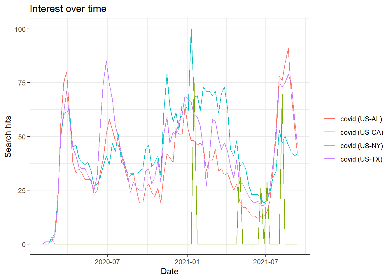

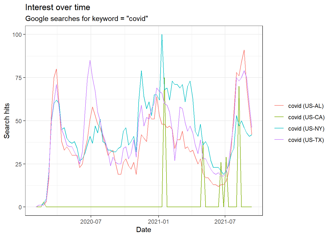
This chart gives us a timeline of daily hits on the keyword “covid” for four different states. The data has been scaled in the following way: First the “hit rate” for a given day and geography is calculated. This is the number of searches on the focal keyword divided by all searches on that day (for that geography). The highest hit rate in the data is then normalized to 100 and everything is rescaled relative to that. In the current example we see that the highest hit rate happened in the state of New York in the beggining of 2021.

The default source for keyword search is Google web searches. You can change this to other Google products. Here is a visualization of the general decline of Kanye West’s career - as exemplified by popularity on YouTube searches in four countries:

## get Youtube query activity for keyword = "kanye" in USA,
## Great Britain, Germany, India
res <- gtrends(c("kanye"),geo=c("US","GB","DE","IN"), gprop = "youtube")
plot(res)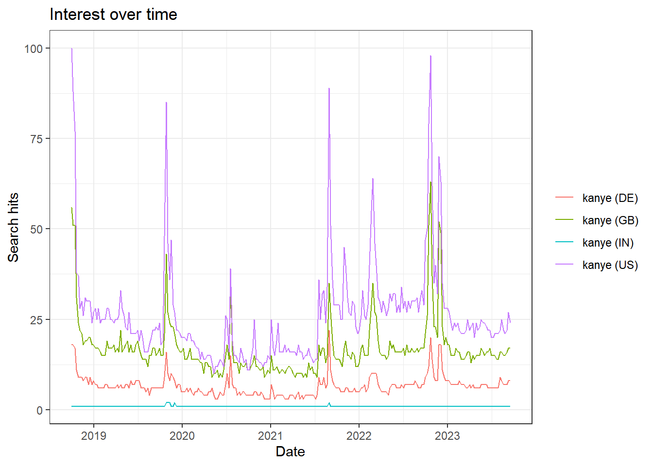

The object returned by the gtrends function contain other information than just the timeline. You can also look at search by city within each of the geographies and search hits on related queries:

library(tidyverse)
## get Google Images query activity for keyword = "chris hemsworth"
## in California and Texas
res <- gtrends(c("chris hemsworth"),geo=c("US-CA","US-TX"), gprop = "images", time = "all")

## plot most popular related queries in California
res$related_queries %>%
  filter(related_queries=="top", geo=="US-CA") %>%
  mutate(value=factor(value,levels=rev(as.character(value))),
         subject=as.numeric(subject)) %>%
  ggplot(aes(x=value,y=subject)) + 
  geom_bar(stat='identity') + 
  coord_flip()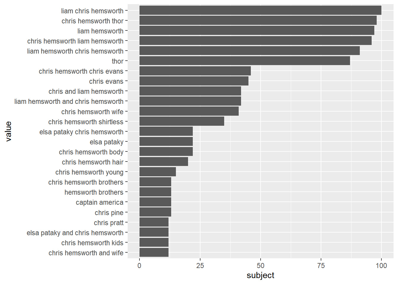

Case Study: Collecting Wikipedia Page Traffic

WWW If you are interested in knowing what topics people pay attention to, an alternative to Google search queries is traffic on Wikipedia pages. How many people visit a certain page in a given day or week or year? Or what are the most frequently visited pages over a certain time period? For this purpose we can use the R package pageviews which makes use of the Wikipedia APIs. It is pretty straightforward to use and you don’t need a personalized API key. Let’s say we want to visualize the traffic to the Wikipedia page for Covid-19 in 2020:

#install.packages("pageviews")
library(tidyverse)
library(pageviews)

CovidViews <-
  article_pageviews(
    project = "en.wikipedia",
    article = "Covid-19",
    user_type = "user",
    start = as.Date("2020-1-1"),
    end = as.Date("2021-9-18")
  )

CovidViews %>%
  ggplot(aes(x=date,y=views)) + geom_line() +
  labs(title = 'Wikipedia Traffic for "Covid-19"')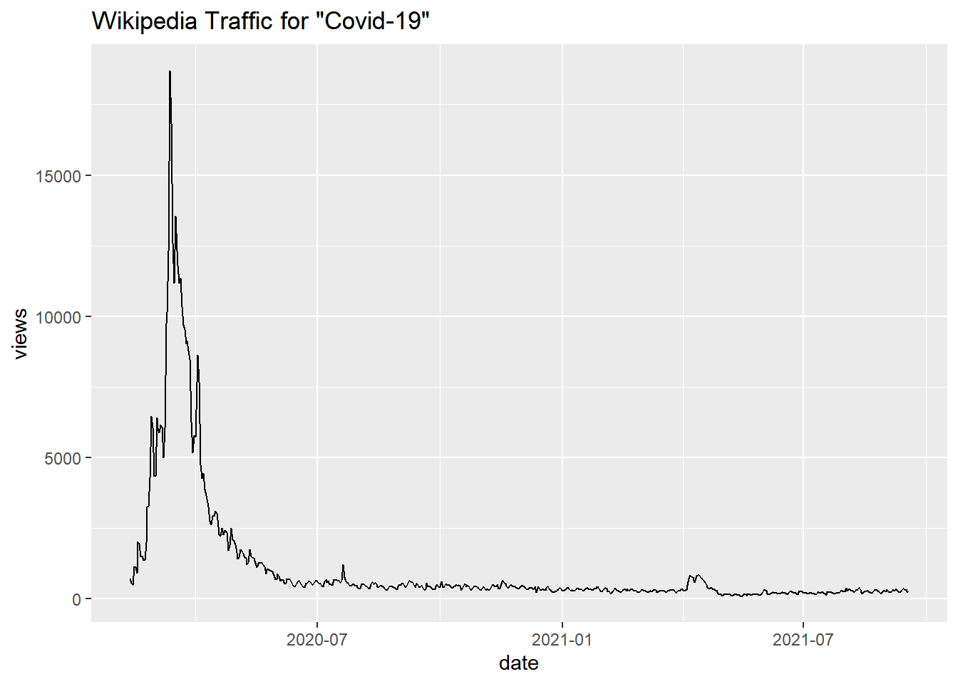

The project option specifies that you want the English language version of Wikipedia (you can just change this to other languages if that’s what you need). You can also ask the API to return the most popular articles over a certain time period:

topArticles <- 
  top_articles(
    project = "en.wikipedia",
    user_type = "user",
    start = as.Date("2021-9-1"),
    end = as.Date("2021-9-18")
  )

The top 5 are

topArticles[1:5,]

    project language           article     access granularity       date rank
1 wikipedia       en         Main_Page all-access         day 2021-09-01    1
2 wikipedia       en    Special:Search all-access         day 2021-09-01    2
3 wikipedia       en Cristiano_Ronaldo all-access         day 2021-09-01    3
4 wikipedia       en             Bible all-access         day 2021-09-01    4
5 wikipedia       en         Cleopatra all-access         day 2021-09-01    5
    views
1 6025547
2 1542394
3  204999
4  152594
5  142509

Note that the first two are the landing page and the search page for Wikipedia. That’s not very interesting. So if we were to plot - say the top 25 - we should probably remove those first:

topArticles %>%
  slice(3:27) %>%
  ggplot(aes(x=fct_reorder(article,views),y=views)) + 
  geom_bar(stat = 'identity') + coord_flip() + 
  labs(title = 'Top Wikipedia Articles from Sept 1-18, 2021.',
       subtitle = 'Note: Main and search page removed',
       x = 'Article')

Case Study: Computer Vision using Google Vision

Both Google and Microsoft have advanced computer vision algorithms available for public use through APIs. Here we will focus on Google’s version (see here for more detail on Google Vision and here for Microsoft’s computer vision API).

For Python There isn’t a library in Python that makes the Google Vision API available in an easy format. Your only option here is therefore to access the low-level API directly. This is not really a problem - just a a little more technical. In the last example below, you can see an example of how to manually call an API from R and Python - without relying on a package/library as an intermediary. There is lots of information available online on how to use the Google VIsion API from Python (here is a good start).

Using R,Computer Vision allows you to learn about the features of a digital image. You can do all of this through an API in R as packaged in the RoogleVision package. Let’s try it out.

We first load the required libraries and - as always - install them first if you haven’t already.

#install.packages("magick") 
#install.packages("googleAuthR") 
#devtools::install_github("cloudyr/RoogleVision")
library(magick)               # library for image manipulation
library(googleAuthR)          # library for authorizing Google cloud access
library(RoogleVision)         # library for Google Vision API calls
library(tidyverse)

First we need to authorize access to Google’s cloud computing platform. You need an account to do this (it is free). Go here to sign up. Once you have an account to create a project, enable billing (they will not charge you) and enable the Google Cloud Vision API (Go to “Dashboard” under “APIs & Services” to do this). Then click on “Credentials” under “APIs & Services” amnd finally “Create credentials” to get your client id and client secret. Once you have obtained these you then call the gar_auth function in the googleAuthR library and you are good to go!

options("googleAuthR.client_id" = "Your Client ID")
options("googleAuthR.client_secret" = "Your Client Secret")

options("googleAuthR.scopes.selected" = c("https://www.googleapis.com/auth/cloud-platform"))
googleAuthR::gar_auth()

You can now call the GoogleVision API with an image. We can read an image into R by using the magick library:

library(magick)
the_pic_file <- 'pics/luna.jpg'
Kpic <- image_read(the_pic_file) 
print(Kpic)

# A tibble: 1 x 7
  format width height colorspace matte filesize density
  <chr>  <int>  <int> <chr>      <lgl>    <int> <chr>  
1 JPEG     623    971 sRGB       FALSE   158927 72x72

Let’s see what Google Vision thinks this is an image of. We use the option “LABEL_DETECTION” to get features of an image:

PicVisionStats = getGoogleVisionResponse(the_pic_file,feature = 'LABEL_DETECTION',numResults = 20)
PicVisionStats

          mid        description     score topicality
1   /m/0bt9lr                Dog 0.9478306  0.9478306
2    /m/0kpmf          Dog breed 0.8999199  0.8999199
3    /m/01lrl          Carnivore 0.8777413  0.8777413
4   /m/07_gml     Working animal 0.8343861  0.8343861
5   /m/03yl64      Companion dog 0.8228148  0.8228148
6  /m/0276krm               Fawn 0.8157332  0.8157332
7   /m/03_pfn              Liver 0.8012283  0.8012283
8   /m/0fbf1m Terrestrial animal 0.7670484  0.7670484
9  /m/0265rtm     Sporting Group 0.7033364  0.7033364
10  /m/02mtq_            Gun dog 0.6918846  0.6918846
11   /m/01z5f            Canidae 0.6805871  0.6805871
12 /m/03yddhn            Borador 0.6777479  0.6777479
13   /m/0cnmr                Fur 0.5919996  0.5919996
14   /m/083vt               Wood 0.5851811  0.5851811
15  /m/02gxqz        Hunting dog 0.5289062  0.5289062
16  /m/01l7qd           Whiskers 0.5127557  0.5127557
17  /m/05q778         Dog collar 0.5078828  0.5078828

The numbers are feature scores with higher being more likely (max of 1). In this case the algorithm does remarkably well. Let’s try another image:

the_pic_file <- 'pics/bike.jpg'
Kpic <- image_read(the_pic_file) 
print(Kpic)

# A tibble: 1 x 7
  format width height colorspace matte filesize density
  <chr>  <int>  <int> <chr>      <lgl>    <int> <chr>  
1 JPEG    1296    972 sRGB       FALSE   249569 72x72

Ok - in this case we get:

          mid                      description     score topicality
1    /m/0199g                          Bicycle 0.9785153  0.9785153
2    /m/0h9mv                             Tire 0.9727893  0.9727893
3    /m/083wq                            Wheel 0.9712469  0.9712469
4  /m/0bpnmk0 Bicycles--Equipment and supplies 0.9673683  0.9673683
5   /m/01bqgn                    Bicycle frame 0.9532196  0.9532196
6   /m/01ms7j                         Crankset 0.9458060  0.9458060
7  /m/0h8n90g                Bicycle wheel rim 0.9441347  0.9441347
8   /m/05y5lj                 Sports equipment 0.9412552  0.9412552
9   /m/01bqk0                    Bicycle wheel 0.9410691  0.9410691
10 /m/0h8p5xc                 Bicycle seatpost 0.9399017  0.9399017
11 /m/0c3vfpc                     Bicycle tire 0.9391636  0.9391636
12 /m/02rqv26                Bicycle handlebar 0.9388900  0.9388900
13 /m/0h8n8m_                      Bicycle hub 0.9371629  0.9371629
14   /m/07yv9                          Vehicle 0.9316994  0.9316994
15  /m/01cwty                         Hub gear 0.9231227  0.9231227
16  /m/03pyqb                     Bicycle fork 0.9182972  0.9182972
17 /m/0h8n973                     Bicycle stem 0.9161927  0.9161927
18 /m/0h8pb3l                  Automotive tire 0.9160876  0.9160876
19 /m/02qwkrn                    Vehicle brake 0.9040849  0.9040849
20 /m/0h8m1ct                Bicycle accessory 0.9003185  0.9003185

Again the algorithm does really well in detecting the features of the image.

You can also use the API for human face recognition. Let’s read in an image of a face:

the_pic_file <- 'images/Karsten4.jpg'
Kpic <- image_read(the_pic_file) 
print(Kpic)

WWW

We now call the API with the option “FACE_DETECTION”:

PicVisionStats = getGoogleVisionResponse(the_pic_file,feature = 'FACE_DETECTION')

The returned object contains a number of different features of the face in the image. For example, we can ask where the different elements of the face are located in the image and plot a bounding box around the actual face:

xs1 = PicVisionStats$fdBoundingPoly$vertices[[1]][1][[1]]
ys1 = PicVisionStats$fdBoundingPoly$vertices[[1]][2][[1]]

xs2 = PicVisionStats$landmarks[[1]][[2]][[1]]
ys2 = PicVisionStats$landmarks[[1]][[2]][[2]]

img <- image_draw(Kpic)
rect(xs1[1],ys1[1],xs1[3],ys1[3],border = "red", lty = "dashed", lwd = 1)
text(xs2,ys2,labels=PicVisionStats$landmarks[[1]]$type,col="red",cex=0.9)

dev.off()
print(img)

WWW

Here we see that the API with great success has identified the different elements of the face. The API returns other features too:

glimpse(PicVisionStats)

Rows: 1
Columns: 15
$ boundingPoly           <df[,1]> <data.frame[1 x 1]>
$ fdBoundingPoly         <df[,1]> <data.frame[1 x 1]>
$ landmarks              <list> [<data.frame[34 x 2]>]
$ rollAngle              <dbl> 3.411922
$ panAngle               <dbl> 3.015293
$ tiltAngle              <dbl> -8.076313
$ detectionConfidence    <dbl> 0.4958495
$ landmarkingConfidence  <dbl> 0.2965677
$ joyLikelihood          <chr> "VERY_UNLIKELY"
$ sorrowLikelihood       <chr> "VERY_UNLIKELY"
$ angerLikelihood        <chr> "VERY_UNLIKELY"
$ surpriseLikelihood     <chr> "LIKELY"
$ underExposedLikelihood <chr> "VERY_UNLIKELY"
$ blurredLikelihood      <chr> "VERY_UNLIKELY"
$ headwearLikelihood     <chr> "VERY_UNLIKELY"

Here we see that the algorithm considers it likely that the face in the image exhibits surprise (but not joy, sorrow or anger). It also considers it likely that the person in the image has headwear (which is clearly wrong in this case).

How about this one?

WWW

the_pic_file <- 'pics/Karsten1.jpg'
PicVisionStats = getGoogleVisionResponse(the_pic_file,feature = 'FACE_DETECTION')
glimpse(PicVisionStats)

Rows: 1
Columns: 15
$ boundingPoly           <df[,1]> <data.frame[1 x 1]>
$ fdBoundingPoly         <df[,1]> <data.frame[1 x 1]>
$ landmarks              <list> [<data.frame[34 x 2]>]
$ rollAngle              <dbl> 3.833999
$ panAngle               <dbl> 3.728436
$ tiltAngle              <dbl> -0.1224614
$ detectionConfidence    <dbl> 0.6391175
$ landmarkingConfidence  <dbl> 0.2326426
$ joyLikelihood          <chr> "VERY_UNLIKELY"
$ sorrowLikelihood       <chr> "POSSIBLE"
$ angerLikelihood        <chr> "VERY_UNLIKELY"
$ surpriseLikelihood     <chr> "VERY_UNLIKELY"
$ underExposedLikelihood <chr> "VERY_UNLIKELY"
$ blurredLikelihood      <chr> "VERY_UNLIKELY"
$ headwearLikelihood     <chr> "VERY_UNLIKELY"

Pretty good!

Querying an API Manually

If you want to query an API for which there is no R package, you need to set up the queries manually. This can be done by use of the GET function in the httr package. The argument to this function will be driven by the protocol of the particular API you are interested in. To find out what this protocol is, you need to look up the API documentation.

Case Study: Collecting Data from The Washington Metropolitan Area Transport Authority

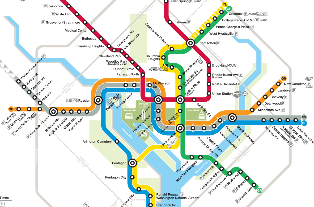WWW The Washington Metropolitan Area Transport Authority has a nice and well documented API. Let’s use this to collect data on the current positions of all buses on a given bus route. To do this you first have to register on their site. You can do that here. You will then be given an API key you can use for data collection.

There are several APIs available for use. Here we will focus on one returning real time bus positions. In the code below we call the API asking for the current position of all buses on the S4 bus route. To get the correct string argument to the get functions below, just look up the documentation on the bus positions API.

PYTHON
R

We can also easily call manual APIs. The bus example above can be replicated in Python as follows:

import pandas as pd
import requests
import json

myApiKey = "your api key"
TheRoute =  "S2"

theURL = "https://api.wmata.com/Bus.svc/json/jBusPositions?RouteID="+TheRoute+"&api_key="+myApiKey

response = requests.get(theURL)
j = response.json()

busPos = j['BusPositions']
df = pd.json_normalize(busPos)

print(df.head())

  VehicleID        Lat  ...          TripEndTime  BlockNumber
0      5467  38.993892  ...  2023-09-27T15:15:00        MS-12
1      5468  38.894533  ...  2023-09-27T15:23:00        MS-16
2      5527  38.987176  ...  2023-09-27T15:27:00        MS-11
3      7341  38.926701  ...  2023-09-27T15:57:00        MC-27
4      5529  38.933454  ...  2023-09-27T15:53:00        MS-09

[5 rows x 13 columns]

The API returns an R list of data that we immediately convert to an R data frame. Finally we plot the results on a nice interactive leaflet map:

library(leaflet)
library(httr)
myApiKey <- "your api key"

## plot current positions of all active busses on route S4
TheRoute <- "S2"
BusGet <- GET(paste0("https://api.wmata.com/Bus.svc/json/jBusPositions?RouteID=",
                     TheRoute,
                     "&api_key=",
                     myApiKey))
BusResult <- content(BusGet)

## convert result to an R data frame
BusResultDF <- do.call(rbind.data.frame,BusResult$BusPositions) 

## plot bus location on an R leaflet map
leaflet(BusResultDF) %>% 
  addTiles() %>%
  addCircles(lng = ~Lon, lat = ~Lat, radius = 200, popup = ~VehicleID)

Warning: package 'httr' was built under R version 4.1.3