usethis::use_course("https://www.dropbox.com/sh/q3w2bvju4lowy4d/AAC_Noadt_lYpSULcnCtcAaJa?dl=1")Summarizing a Corpus
Text data is messy and to make sense of it you often have to clean it a bit first. For example, do you want “Tuesday” and “Tuesdays” to count as separate words or the same word? Most of the time we would want to count this as the same word. Similarly with “run” and “running”. Furthermore, we often are not interested in including punctuation in the analysis - we just want to treat the text as a “bag of words”. There are libraries in R that will help you do this.
You can download the code and data for this module by using this dropbox link: https://www.dropbox.com/sh/q3w2bvju4lowy4d/AAC_Noadt_lYpSULcnCtcAaJa?dl=0. If you are using Rstudio you can do this from within Rstudio:
In the following let’s look at Yelp reviews of Las Vegas hotels:
library(tidyverse)
reviews <- read_cvs('data/vegas_hotel_reviews.csv')
business <- read_csv('data/vegas_hotel_info.csv')
This data contains customer reviews of 18 hotels in Las Vegas. In addition to text, each review also contain a star rating from 1 to 5. Let’s see how the 18 hotels fare on average in terms of star ratings:
library(scales)
library(lubridate)

reviews %>%
  left_join(select(business,business_id,name),
             by='business_id') %>%
  group_by(name) %>%
  summarize(n = n(),
            mean.star = mean(as.numeric(stars))) %>%
  arrange(desc(mean.star)) %>%
  ggplot() +
  geom_point(aes(x=reorder(name,mean.star),y=mean.star,size=n))+
  coord_flip() +
  ylab('Mean Star Rating (1-5)') +
  xlab('Hotel')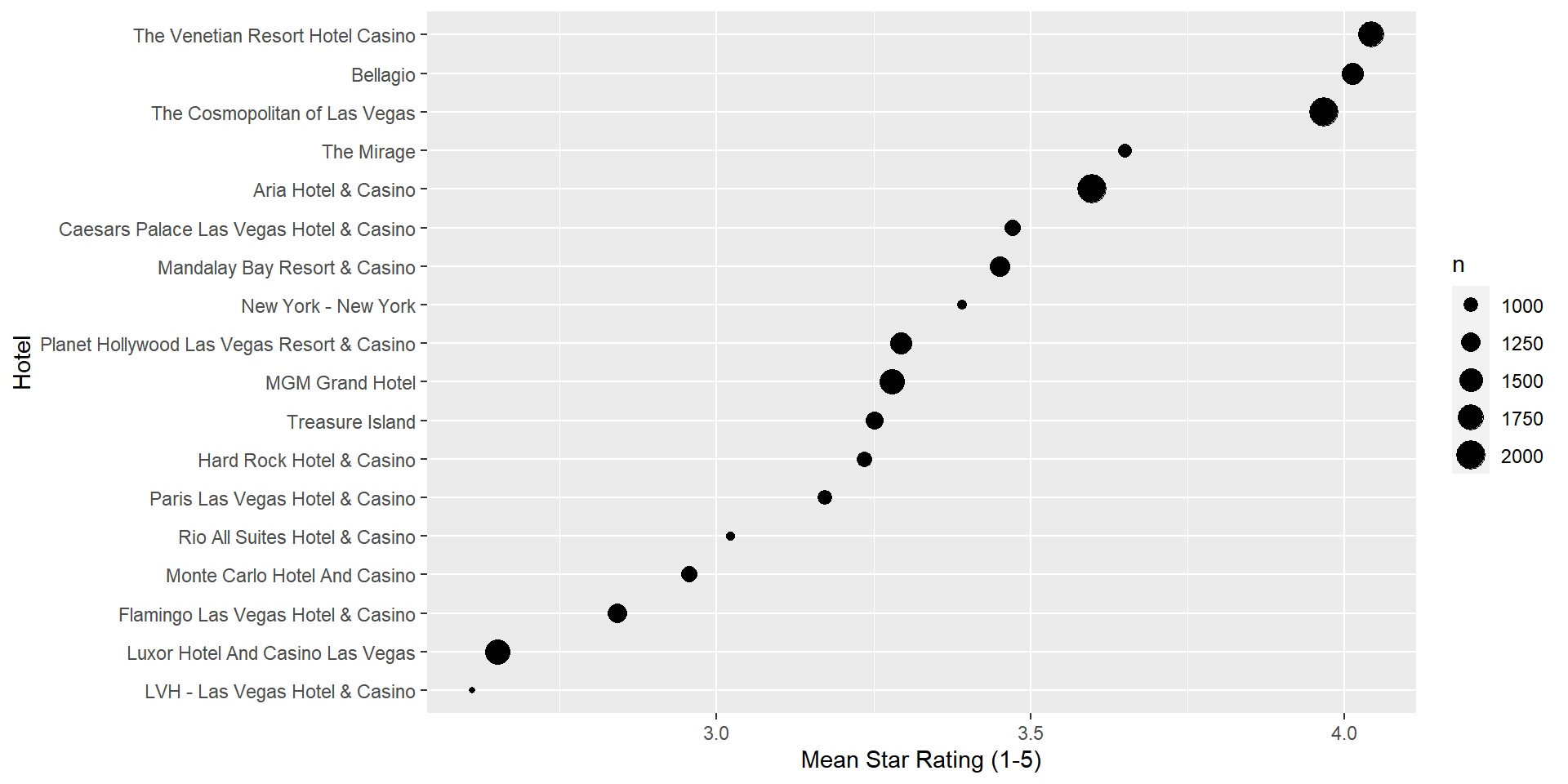
So The Venetian, Bellagio and The Cosmopolitan are clearly the highest rated hotels, while Luxor and LVH are the lowest rated. Ok, but what is behind these ratings? What are customers actually saying about these hotels? This is what we can hope to find through a text analysis.
Basic Text Analysis in R
Constructing a Document Term Matrix
In the following we will make use of two libraries for text mining:
## install packages
install.packages(c("wordcloud","tidytext"))  ## only run once
library(tidytext)
library(wordcloud)
Simple text summaries is often based on the document term matrix. This is an array where each row corresponds to a document and each column corresponds to a word. The entries of the array are simply counts of how many times a certain word occurs in a certain document. Let’s look at a simple example:
example <- data.frame(doc_id = c(1:4),
                      text=c("I have a brown dog. My dog loves walks.",
                       "My dog likes food.",
                       "I like food.",
                       "Some dogs are black."),
                      stringsAsFactors = F)
This data contains four documents. The first document contains 8 unique words (or “terms”). The word “brown” occurs once while “dog” occurs twice. We can create document-term counts using the tidytext’s library unnest_tokens and then a simple count:
example %>%
  unnest_tokens(word,text) %>%
  count(doc_id,word)
doc_id word n
1 1 a 1
2 1 brown 1
3 1 dog 2
4 1 have 1
5 1 i 1
6 1 loves 1
7 1 my 1
8 1 walks 1
9 2 dog 1
10 2 food 1
11 2 likes 1
12 2 my 1
13 3 food 1
14 3 i 1
15 3 like 1
16 4 are 1
17 4 black 1
18 4 dogs 1
19 4 some 1This data contains four documents. The first document contains 8 unique words (or “terms”). The word “brown” occurs once while “dog” occurs twice. Note that punctuation is removed and lower-casing is done automatically.
We are usually performing text summaries with the goal of understanding what a document or set of documents are about. To this end many of the often used words in the English language are useless - words such as the, and, it and so on. These words are called “stop words” and we can remove them automatically by using an anti_join :
example %>%
  unnest_tokens(word,text) %>%
  count(doc_id,word) %>%
  anti_join(stop_words)
doc_id word n
1 1 brown 1
2 1 dog 2
3 1 loves 1
4 1 walks 1
5 2 dog 1
6 2 food 1
7 2 likes 1
8 3 food 1
9 4 black 1
10 4 dogs 1We now have a more distilled and interesting representation of each document. Let’s try this out on some real data - the hotel reviews above. Suppose we are interersted in summarizing the reviews for the Aria hotel:
aria.id <-  filter(business,
        name=='Aria Hotel & Casino')$business_id
aria.reviews <- filter(reviews,
                       business_id==aria.id)


AriaTidy <- aria.reviews %>%
  select(review_id,text,stars) %>%
  unnest_tokens(word,text)

AriaFreqWords <- AriaTidy %>%
  count(word)
Let’s plot the top words:
AriaFreqWords %>%
  top_n(25) %>%
  ggplot(aes(x=fct_reorder(word,n),y=n)) + geom_bar(stat='identity') +
  coord_flip() + theme_bw()+
  labs(title='Top 25 Words in Aria Reviews',
       x='Count',
       y= 'Word')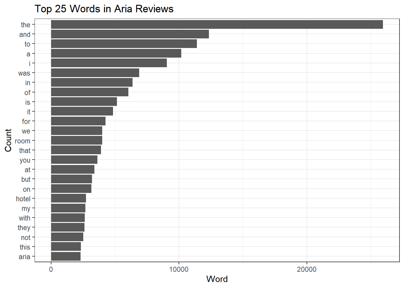
ok - so here we see the problem with stop words. Let’s remove them:
AriaFreqWords %>%
  anti_join(stop_words) %>%
  top_n(25) %>%
  ggplot(aes(x=fct_reorder(word,n),y=n)) + geom_bar(stat='identity') +
  coord_flip() + theme_bw()+
  labs(title='Top 25 Words in Aria Reviews',
       subtitle = 'Stop Words Removed',
       x='Count',
       y= 'Word')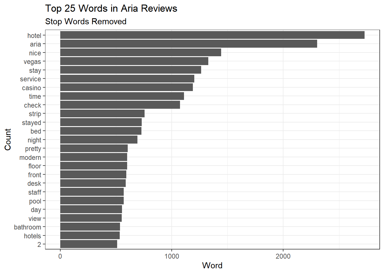
Much better! But how do these top words vary with the rating of the underlying reviews? This is an easy extension:
AriaFreqWordsByRating <- AriaTidy %>%
  count(stars,word)
AriaFreqWordsByRating %>%
anti_join(stop_words) %>%
group_by(stars) %>%
top_n(20) %>%
ggplot(aes(x=reorder_within(word,n,stars),
y=n,
fill=stars)) +
geom_bar(stat='identity') +
coord_flip() +
scale_x_reordered() +
facet_wrap(~stars,scales = 'free',nrow=1) +
theme_bw() +
theme(legend.position = "none")+
labs(title = 'Top Words by Review Rating',
subtitle = 'Stop words removed',
x = 'Word',
y = 'Count')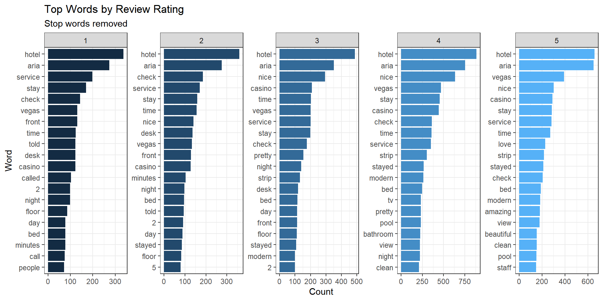
Here we can begin to see what is behind low rated experiences and high rated experiences.
A typical visualization of document term arrays are word clouds. These can easily be done in R:
topWords <- AriaFreqWords %>%
  anti_join(stop_words) %>%
  top_n(100)

wordcloud(topWords$word,
           topWords$n,
           scale=c(5,0.5),
           colors=brewer.pal(8,"Dark2"))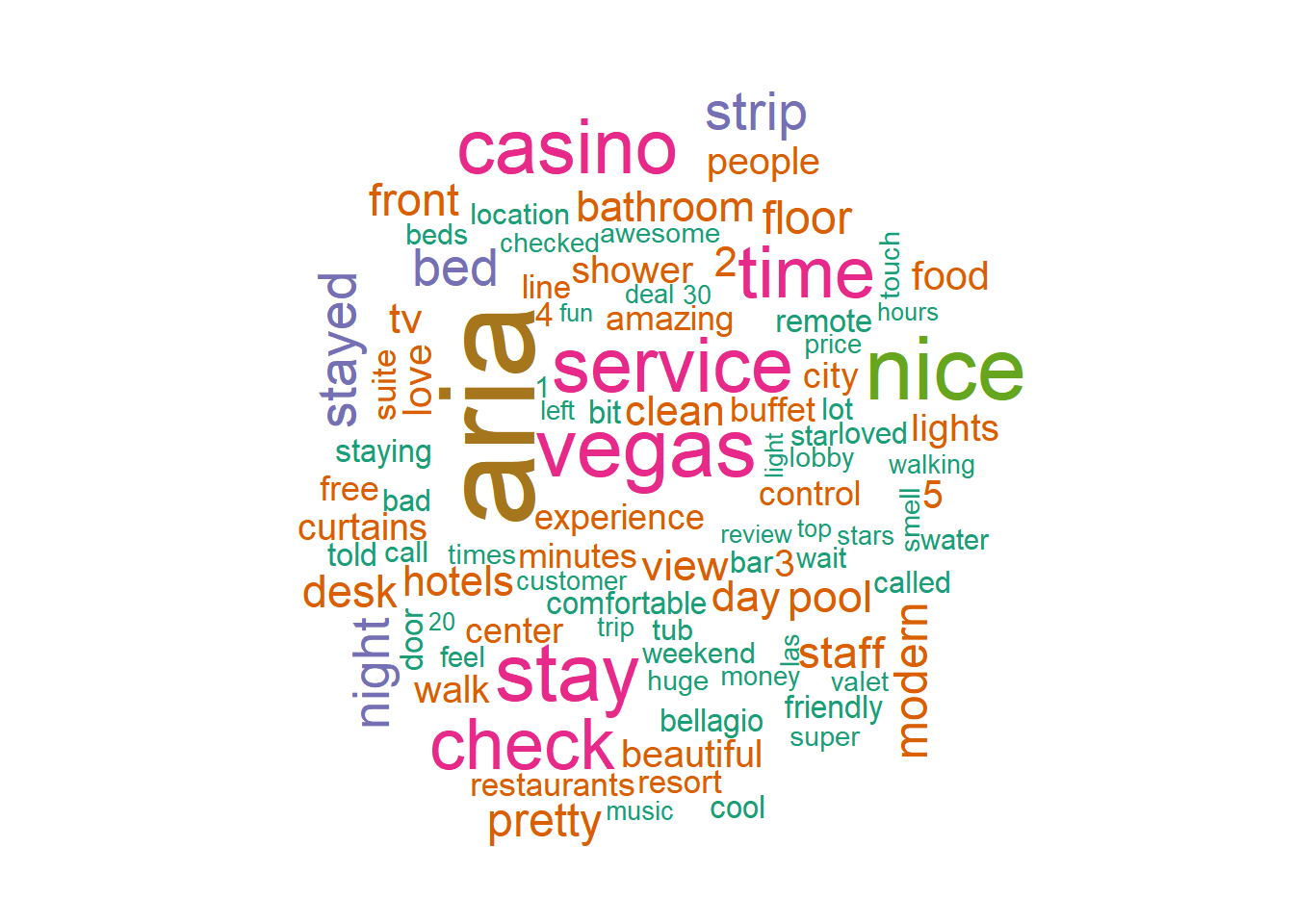
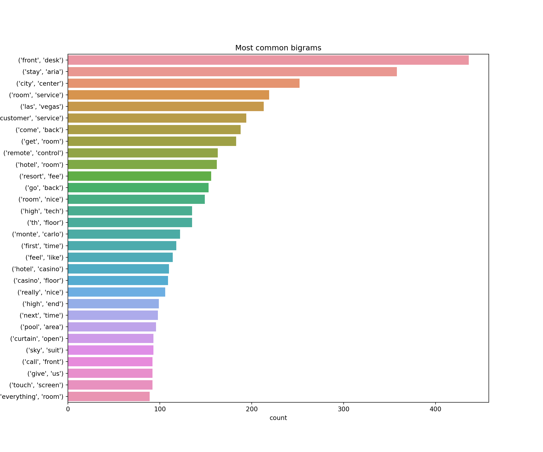
Above we looked at terms in isolation. Sometimes we may want to summarize terms two at a time. These are called “bi-grams”:
aria.reviews %>%
  select(review_id,text) %>%
  unnest_tokens(bigram,text,token="ngrams",n=2) %>%
  count(bigram) %>%
  top_n(40) %>%
  ggplot(aes(x=fct_reorder(bigram,n),y=n)) + geom_bar(stat='identity') +
  coord_flip() +
  labs(title="Top Bi-grams",
       x = "Counts",
       y = "Terms")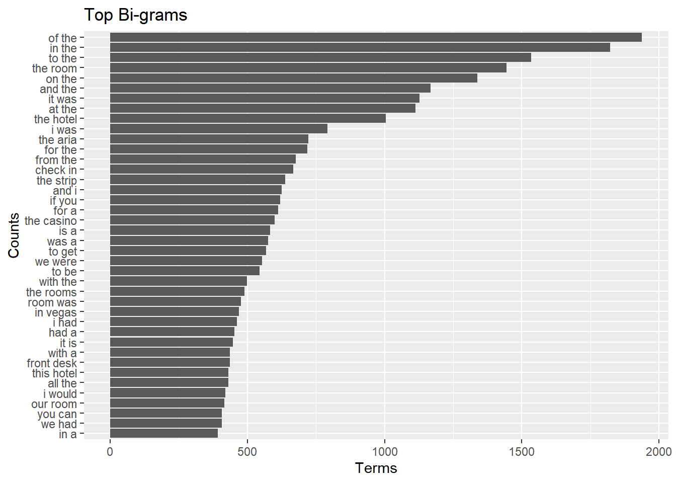
All of the above analyses looked at overall term frequencies. Sometimes we may have a different objective: What is one given document about? The default metric for this question is a document’s Term-Frequency-Inverse Document-Frequency (TF-IDF). A word’s TF-IDF is a measure of how important a word is to a document. It is calculated as \[ \text{TF}(\text{word}) = \frac{\text{number of times word appears in document}}{\text{total number of words in document}} \] \[ \text{IDF}(\text{word}) = \log_e \frac{ \text{total number of documents}}{\text{Number of documents with word in it}} \] \[ \text{TF-IDF}(\text{word}) = \text{TF}(\text{word}) \times \text{IDF}(\text{word}) \]
Words with high TF-IDF in a document will tend to be words that are rare (when compared to other documents) but not too rare. In this way they are informative about what the document is about! We can easily calculate TF-IDF using bind_tf_idf:
tidyReviews <- aria.reviews %>%
  select(review_id,text) %>%
  unnest_tokens(word, text) %>%
  count(review_id,word)

minLength <- 200  # focus on long reviews
tidyReviewsLong <- tidyReviews %>%
  group_by(review_id) %>%
  summarize(length = sum(n)) %>%
  filter(length >= minLength)

tidyReviewsTFIDF <- tidyReviews %>%
  filter(review_id %in% tidyReviewsLong$review_id) %>%
  bind_tf_idf(word,review_id,n) %>%
  group_by(review_id) %>%
  arrange(desc(tf_idf)) %>%
  slice(1:15) %>% # get top 15 words in terms of tf-idf
  ungroup() %>%
  mutate(xOrder=n():1) %>%  # for plotting
  inner_join(select(aria.reviews,review_id,stars),by='review_id')  # get star ratings
Here is a plot of the top TF-IDF words for 12 reviews:
nReviewPlot <- 12
plot.df <- tidyReviewsTFIDF %>%
  filter(review_id %in% tidyReviewsLong$review_id[1:nReviewPlot])

plot.df %>%
  mutate(review_id_n = as.integer(factor(review_id))) %>%
  ggplot(aes(x=xOrder,y=tf_idf,fill=factor(review_id_n))) +
  geom_bar(stat = "identity", show.legend = FALSE) +
  facet_wrap(~ review_id_n,scales='free') +
  scale_x_continuous(breaks = plot.df$xOrder,
                     labels = plot.df$word,
                     expand = c(0,0)) +
  coord_flip()+
  labs(x='Word',
       y='TF-IDF',
       title = 'Top TF-IDF Words in Reviews of Aria',
       subtitle = paste0('Based on first ',
                         nReviewPlot,
                         ' reviews'))+
  theme(legend.position = "none")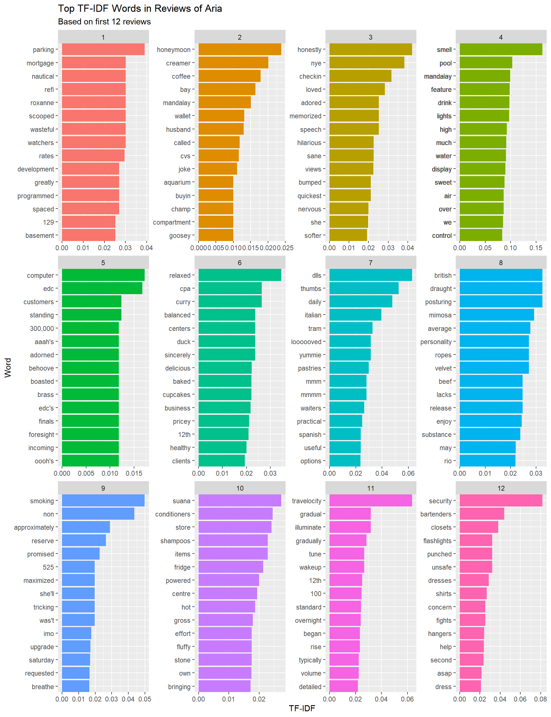
One can think of these as “key-words” for each review.
Aria v2.0
If you want to try out a much bigger database of Aria reviews, you can use the data in the file AriaReviewsTrip.rds. This contains 10,905 reviews of the Aria hotel scraped from Tripadvisor.
aria <- read_csv('data/AriaReviewsTrip.csv') %>%
  rename(text = reviewText)

meta.data <- aria %>%
  select(reviewID,reviewRating,date,year.month.group)
With this sample size you can do more in-depth analyses. For example, how do word frequencies change over time? In the following we focus on the terms “buffet”,“pool” and “staff”. We calculate the relative frequency of these three terms for each month (relative to the total number of terms used that month).
ariaTidy <- aria %>%
  select(reviewID,text) %>%
  unnest_tokens(word,text) %>%
  count(reviewID,word) %>%
  inner_join(meta.data,by="reviewID")

total.terms.time <- ariaTidy %>%
  group_by(year.month.group) %>%
  summarize(n.total=sum(n))

## for the legend
a <- 1:nrow(total.terms.time)
b <- a[seq(1, length(a), 3)]

ariaTidy %>%
  filter(word %in% c("pool","staff","buffet")) %>%
  group_by(word,year.month.group) %>%
  summarize(n = sum(n)) %>%
  left_join(total.terms.time, by='year.month.group') %>%
  ggplot(aes(x=year.month.group,y=n/n.total,color=word,group=word)) +
  geom_line() +
  facet_wrap(~word)+
  theme(axis.text.x = element_text(angle = 90, hjust = 1))+
  scale_x_discrete(breaks=as.character(total.terms.time$year.month.group[b]))+
  scale_y_continuous(labels=percent)+xlab('Year/Month')+
  ylab('Word Frequency relative to Month Total')+
  ggtitle('Dynamics of Word Frequency for Aria Hotel')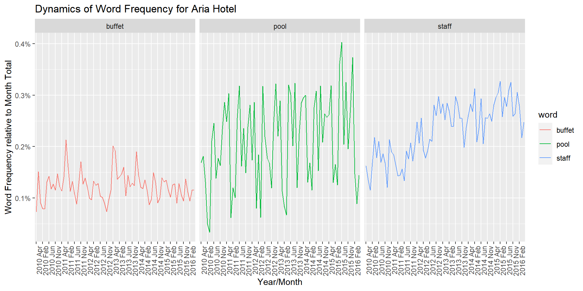
We see three different patterns for the relative frequencies: “buffet” is used in a fairly stable manner over this time period, while “pool” displays clear seasonality, rising in popularity in the summer months. Finally, we see an upward trend in the use of “staff”.
We can try a similar analysis where consider word frequency dynamics for different satisfaction segments:
aria.tidy2 <- ariaTidy %>%
  mutate(year = year(date),
         satisfaction = fct_recode(factor(reviewRating),
                                   "Not Satisfied"="1",
                                   "Not Satisfied"="2",
                                   "Neutral"="3",
                                   "Neutral"="4",
                                   "Satisfied"="5"))

total.terms.rating.year <- aria.tidy2 %>%
  group_by(satisfaction,year) %>%
  summarize(n.total = sum(n))


aria.tidy2 %>%
  filter(word %in% c("pool","staff","buffet","food","wait","casino","line","check","clean")) %>%
  group_by(satisfaction,year,word) %>%
  summarize(n = sum(n)) %>%
  left_join(total.terms.rating.year, by=c('year','satisfaction')) %>%
  ggplot(aes(x=year,y=n/n.total,color=satisfaction,group=satisfaction)) +
  geom_line(size=1,alpha=0.25) + geom_point() +
  facet_wrap(~word,scales='free')+
  theme(axis.text.x = element_text(angle = 90, hjust = 1))+
  scale_y_continuous(labels=percent)+xlab('Year')+
  ylab('Word Frequency relative to Month Total')+
  labs(title='Dynamics of Word Frequency for Aria Hotel',
       subtitle='Three Satisfaction Segments')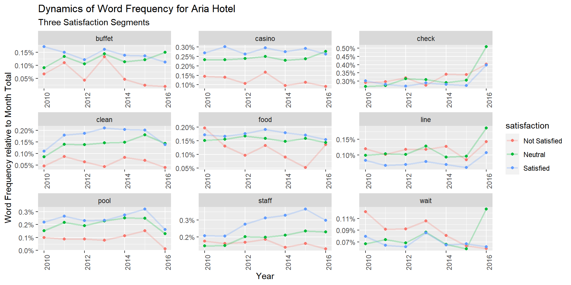
Basic Text Analysis in Python
The most popular library for basic text analysis in Python is the NLTK library (Natural Language Tool Kit). We start by loading the required libraries and functions. We also need to download the dictionaries we will be using (you only need to do this once):
import nltk
from nltk.probability import FreqDist
from nltk.tokenize import RegexpTokenizer
from nltk.stem import WordNetLemmatizer
import string
from nltk.corpus import stopwords
from nltk.util import ngrams
import pandas as pd
import re  # for working with regular expressions
import matplotlib.pyplot as plt
import seaborn as sns
#nltk.download('punkt')       # only need to run this once
#nltk.download('stopwords')   # only need to run this once
#nltk.download('wordnet')     # only need to run this once
#nltk.download('omw-1.4')
lang="english"
We will use the same data as above and focus on the Aria hotel reviews:
reviews = pd.read_csv('../data/vegas_hotel_reviews.csv')
business = pd.read_csv('../data/vegas_hotel_info.csv')
ariaID = "JpHE7yhMS5ehA9e8WG_ETg"
ariaReviews = reviews[reviews.business_id==ariaID]Ok - now we are good to go. Let’s start by lower casing all words and remove punctuation and other non-word characters. We concatenate all the reviews into one long list - then we can do word frequencies on that:
ariaReviewsList = [re.sub("[^\w ]",  " " , x.lower()) for x in ariaReviews['text']]
ariaReviewsStr = ' '.join(ariaReviewsList)
print(ariaReviewsStr[:100])
they likely have some issues to work out but they are a new establishment the trend here as evideNext let’s create tokens - here we set up our tokenizer to keep only tokens with words that are at least two letters long:
tokeniser = RegexpTokenizer(r'[A-Za-z]{2,}')
ariaReviewsTokenized = tokeniser.tokenize(ariaReviewsStr)
print(ariaReviewsTokenized[:100])
['they', 'likely', 'have', 'some', 'issues', 'to', 'work', 'out', 'but', 'they', 'are', 'new', 'establishment', 'the', 'trend', 'here', 'as', 'evidenced', 'by', 'the', 'wynn', 'is', 'non', 'theming', 'one', 'concern', 'that', 'some', 'might', 'have', 'is', 'that', 'the', 'aria', 'and', 'city', 'center', 'look', 'nothing', 'like', 'vegas', 'stayed', 'one', 'night', 'at', 'aria', 'on', 'opening', 'night', 'and', 'checked', 'out', 'most', 'of', 'the', 'bars', 'and', 'common', 'areas', 'in', 'the', 'place', 'the', 'room', 'was', 'quite', 'nice', 'and', 'very', 'high', 'tech', 'like', 'the', 'rest', 'of', 'the', 'hotel', 'decor', 'is', 'muted', 'and', 'brownish', 'walking', 'in', 'the', 'curtains', 'open', 'to', 'do', 'reveal', 'of', 'the', 'view', 'over', 'the', 'strip', 'bellagio', 'is', 'few', 'buildings']We can now count words (or - we should say - tokens). Here are the most 10 frequent tokens:
fdist = FreqDist(ariaReviewsTokenized)
fdist.most_common(10)
[('the', 25948), ('and', 12337), ('to', 11406), ('was', 6888), ('in', 6374), ('of', 6042), ('it', 5885), ('is', 5155), ('for', 4269), ('we', 4123)]Alright - here we have the same problem as in the R version so let’s remove the stop words:
stop_words=set(stopwords.words("english"))
ariaReviewsTokenizedStop = [word for word in ariaReviewsTokenized if not word in stop_words]
fdistStop = FreqDist(ariaReviewsTokenizedStop)
fdistStop.most_common(10)
[('room', 4000), ('hotel', 2750), ('aria', 2379), ('like', 1520), ('nice', 1443), ('vegas', 1337), ('get', 1318), ('one', 1282), ('stay', 1264), ('great', 1207)]Better! As always in Python it is better to put frequently used operations into functions. Let’s do that and then find the top 30 most frequent non-stopword tokens and then plot them:
def process_raw_text(text):
    # Tokenize words
    tokeniser = RegexpTokenizer(r'[A-Za-z]{2,}')
    tokens = tokeniser.tokenize(text)

    # Lowercase tokens
    tokens_lower = [token.lower() for token in tokens]

    # Remove stopwords
    clean = [token for token in tokens_lower if token not in stop_words]
    return clean

def frequent_tokens(corpus, n):
    # Preprocess each document
    documents = [process_raw_text(document) for document in corpus]

    # get all tokens and put into one long list
    allTokens = [document for document in documents]
    allTokens_flat = [item for sublist in allTokens for item in sublist]

    # Find frequency of ngrams
    freq_dist = FreqDist(allTokens_flat)
    top_freq = freq_dist.most_common(n)
return pd.DataFrame(top_freq, columns=["token", "count"])data=frequent_tokens(ariaReviews['text'],30)
print(data) token count
0 room 4000
1 hotel 2750
2 aria 2379
3 like 1520
4 nice 1443
5 vegas 1337
6 get 1318
7 one 1282
8 stay 1264
9 great 1207
10 service 1201
11 casino 1198
12 rooms 1175
13 would 1147
14 time 1111
15 check 1075
16 really 1008
17 good 928
18 place 904
19 us 903
20 also 854
21 back 794
22 even 780
23 strip 758
24 stayed 731
25 everything 731
26 bed 727
27 night 701
28 go 698
29 got 677plt.figure(figsize=(12,10))
sns.barplot(x="count", y="token", data=data)
plt.title("Most common tokens")
plt.show()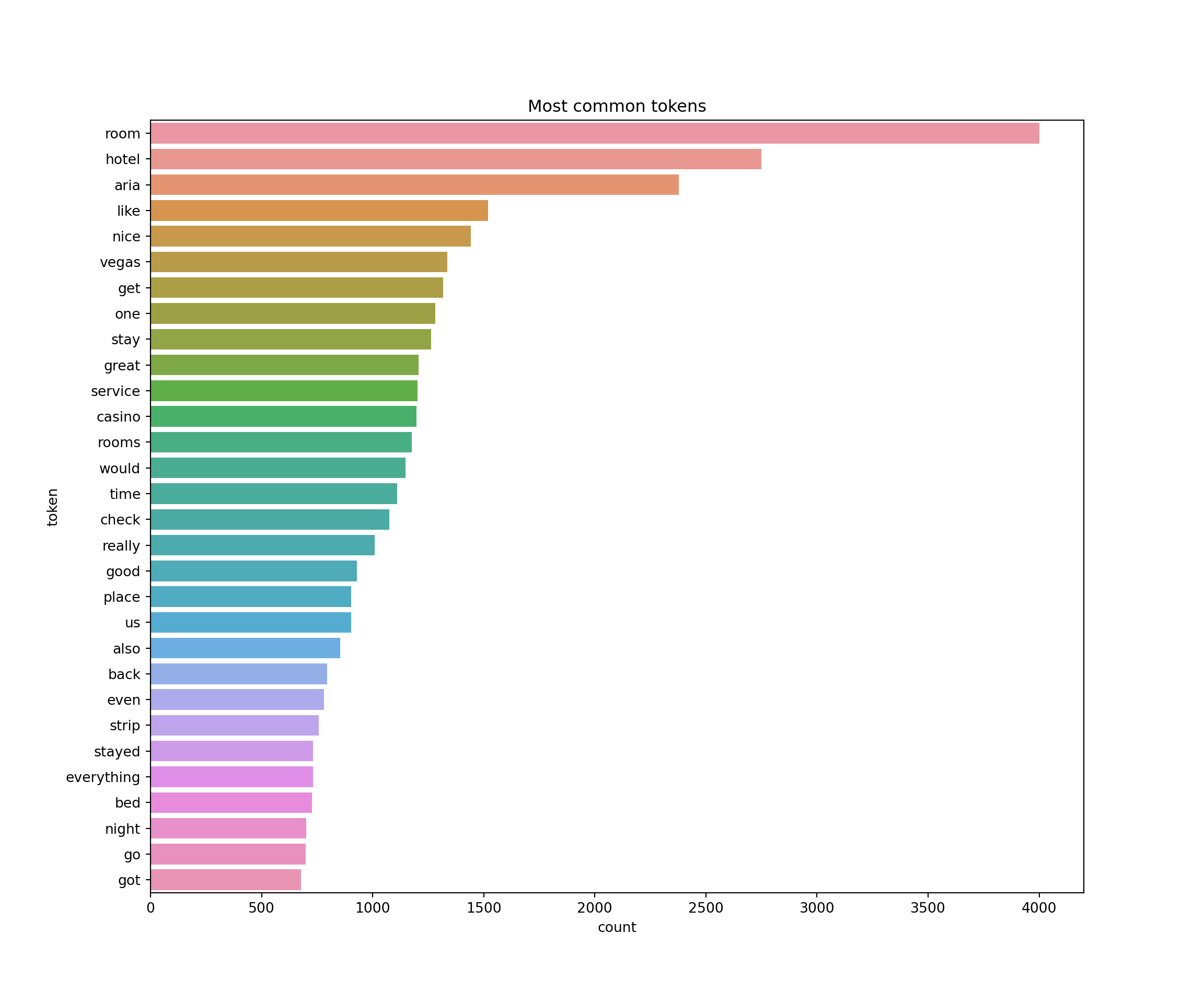
Looks good! Now let’s advance this a little. First of all, when we count words do we really want to treat “room” and “rooms” as different words? How about “meeting” and “meet”? For most purposes we don’t want to treat these differently. The process of finding the root word of a word is called lemmatization and the root words are called lemmas. Below we add lemmatization to the text cleaning function. Second, we might want to extract with single tokens (unigrams) or two tokens (bigrams) or more. We can use the ngrams function for that and we add that to our frequency function:
def process_raw_text(text):
    # Tokenize words
    tokeniser = RegexpTokenizer(r'[A-Za-z]{2,}')
    tokens = tokeniser.tokenize(text)

    # Lowercase, lemmatize and remove stopwords
    lemmatizer = WordNetLemmatizer()
    lemmas = [lemmatizer.lemmatize(token.lower(), pos='v') for token in tokens]
    lemmas = [token.lower() for token in lemmas]

    clean = [lemma for lemma in lemmas if lemma not in stop_words]
    return clean

def frequent_ngram(corpus, ngram, n):
    # Preprocess each document
    documents = [process_raw_text(document) for document in corpus]

    # Find ngrams per document and put into one long list
    n_grams = [list(ngrams(document, ngram)) for document in documents]
    n_grams_flat = [item for sublist in n_grams for item in sublist]

    # get frequencies of ngrams
    freq_dist = FreqDist(n_grams_flat)
    top_freq = freq_dist.most_common(n)
    return pd.DataFrame(top_freq, columns=["ngram", "count"])
Ok - now let’s try this out for unigrams and bigrams and plot the results:
data_unigrams=frequent_ngram(ariaReviews['text'],1,30)
data_bigrams=frequent_ngram(ariaReviews['text'],2,30)plt.figure(figsize=(12,10))
sns.barplot(x="count", y="ngram", data=data_unigrams)
plt.title("Most common unigrams")
plt.show()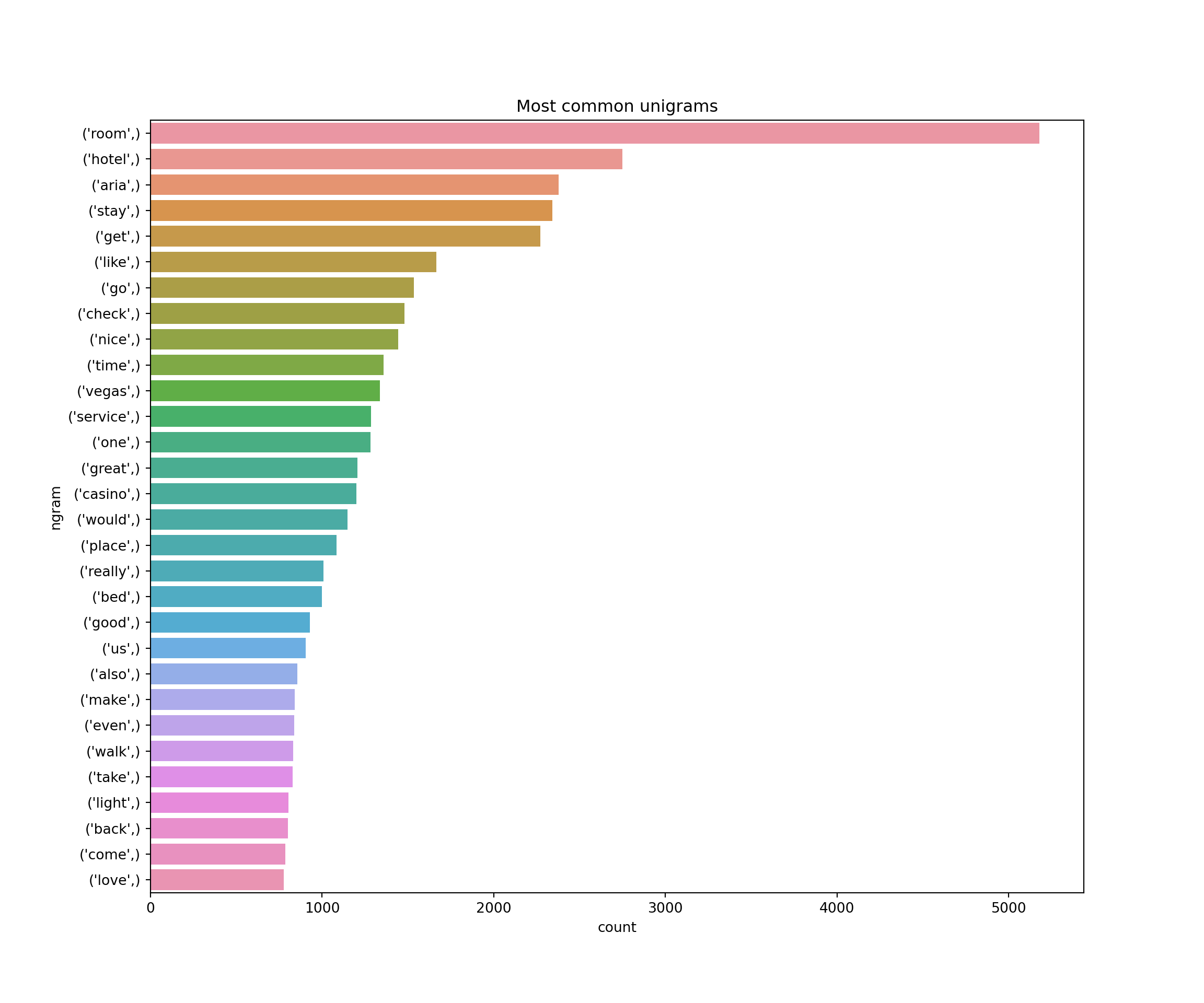
plt.figure(figsize=(12,10))
sns.barplot(x="count", y="ngram", data=data_bigrams)
plt.title("Most common bigrams")
plt.show()