usethis::use_course("https://www.dropbox.com/sh/4209h1zxaafjpv2/AAA8N57nFHz1MhDd6axnzu-Ra?dl=1")Managing Data in Python and R
Raw data is typically not available as R data files. If your data has been extracted from a database, you will most likely receive it as flat text files, e.g., csv files. Data recording web activity is often stored in a format called json. In this section we will look at how to easily read data files into memory.
You can download the code and data for this module by using this dropbox link: https://www.dropbox.com/sh/4209h1zxaafjpv2/AAA8N57nFHz1MhDd6axnzu-Ra?dl=0. If you are using Rstudio you can do this from within Rstudio:
Loading CSV Files in into Python and R
One of the most popular files formats for exchanging and storing data are comma-separated values files or CSV files. This is a left-over from the days of spreadsheets and is not a particularly efficient storage format for data but it is still widely used in businesses and other organizations. In a CSV file the first row contains the variable names. The next row contains the observations for the first record, separated by commas and then the next row for the second record and so on.
Case Study: Airbnb Data
 Let’s look at some data from the peer-to-peer house rental service Airbnb. There are different ways to obtain data on Airbnb listings. The most direct way is, of course, by working for Airbnb so you can access their servers directly. Alternatively, you can scrape data of the Airbnb website (as long as it doesn’t violate the terms of service of the site) or obtain the data through third parties. Here we will follow the last approach. The website Inside Airbnb provides Airbnb data from most of the major markets where Airbnb operate. Let’s focus on the San Diego listings. The data for each market is provided on the Get the Data page of the website. Go there and scroll down to San Diego. There are several files available - let’s focus on the “detailed listings” data in the file listings.csv.gz. This is a compressed CSV file. Download this file and unzip the compressed file - this will generate a file called listings.csv (note: this has already been done in the associated project and the files can be found in the data folder).
CSV files are straightforward to read into Python. The easiest method is to simply se the read_csv function in polars:
import polars as pl

SDlistings = pl.read_csv("data/listings.csv", dtypes={"license": str})
print(SDlistings.shape)
(12404, 74)Just like R, Polars will try to guess what the format is for each column of the data file. Here we forced the “license” column to be a string (you can try without doing this to see what happens)
Alternatively, we can read the same data from a compressed file or directly from the web:
SDlistings = pl.read_csv("data/listings.csv.gz", dtypes={"license": str})
print(SDlistings.shape)
(12404, 74)# read directly online
file_link = "http://data.insideairbnb.com/united-states/ca/san-diego/2020-07-27/data/listings.csv.gz"
SDlistings = pl.read_csv(file_link, dtypes={"license": str})
print(SDlistings.shape)(12404, 74)CSV files are straightforward to read into Python. The easiest method is to simply ise the read_csv function in pandas:
import pandas as pd

SDlistings = pd.read_csv("data/listings.csv", dtype={"license": "string"})
print(SDlistings.shape)
(12404, 74)Just like R, Python (using the pandas library) will try to guess what the format is for each column of the data file. Here we forced the “license” column to be a string (you can try without doing this to see what happens)
Alternatively, we can read the same data from a compressed file or directly from the web:
SDlistings = pl.read_csv("data/listings.csv.gz", dtypes={"license": str})
print(SDlistings.shape)
(12404, 74)# read directly online
file_link = "http://data.insideairbnb.com/united-states/ca/san-diego/2020-07-27/data/listings.csv.gz"
SDlistings = pl.read_csv(file_link, dtypes={"license": str})
print(SDlistings.shape)CSV files are straightforward to read into R. The fastest method for doing so is using the read_csv function contained in the tidyverse library set so let’s load this library:
library(tidyverse)Now that you have downloaded the required file you can read the data into R’s memory by using the read_csv command:
SDlistings <- read_csv(file = "data/listings.csv")This will create a data frame in R’s memory called SDlistings that will contain the data in the CSV file. This code assumes that the downloaded (and uncompressed) CSV file is located in the “data” sub-folder of the current working directory. If the file is located somewhere else that is not a sub-folder of your working directory, you need to provide the full path to the file so R can locate it, for example:
SDlistings <- read_csv(file = "C:/Mydata/airbnb/san_diego/listings.csv")Our workflow above was to first first download the compressed file, then extract it and then read in the uncompressed file. You actually don’t need to uncompress the file first - just can just read in the compressed file directly:
SDlistings <- read_csv(file = "C:/Mydata/airbnb/san_diego/listings.csv.gz")This is a huge advantage since you can then store the raw data in compressed format.
If you are online you don’t even need to download the file first - R can read it off the source website directly:
file.link <- "http://data.insideairbnb.com/united-states/ca/san-diego/2020-07-27/data/listings.csv.gz"
SDlistings <- read_csv(file = file.link)
Once you have read in raw data to R, it is highly recommended to store the original data in R’s own compressed format called rds. R can read in these files extremely fast. This way you only need to read in the original data file once. So the recommended workflow would be
## only run this section once! ------------------------------------------------------------------------
file.link <- "http://data.insideairbnb.com/united-states/ca/san-diego/2020-07-27/data/listings.csv.gz"
SDlistings <- read_csv(file = file.link) # read in raw data
saveRDS(SDlistings, file = "data/listingsSanDiego.rds") # save as rds file


## start here after you have executed the code above once ---------------------------------------------
AirBnbListingsSD <- read_rds("data/listingsSanDiego.rds") # read in rds file
What fields are available in this data? You can see this as
names(AirBnbListingsSD) [1] "id"
[2] "listing_url"
[3] "scrape_id"
[4] "last_scraped"
[5] "name"
[6] "description"
[7] "neighborhood_overview"
[8] "picture_url"
[9] "host_id"
[10] "host_url"
[11] "host_name"
[12] "host_since"
[13] "host_location"
[14] "host_about"
[15] "host_response_time"
[16] "host_response_rate"
[17] "host_acceptance_rate"
[18] "host_is_superhost"
[19] "host_thumbnail_url"
[20] "host_picture_url"
[21] "host_neighbourhood"
[22] "host_listings_count"
[23] "host_total_listings_count"
[24] "host_verifications"
[25] "host_has_profile_pic"
[26] "host_identity_verified"
[27] "neighbourhood"
[28] "neighbourhood_cleansed"
[29] "neighbourhood_group_cleansed"
[30] "latitude"
[31] "longitude"
[32] "property_type"
[33] "room_type"
[34] "accommodates"
[35] "bathrooms"
[36] "bathrooms_text"
[37] "bedrooms"
[38] "beds"
[39] "amenities"
[40] "price"
[41] "minimum_nights"
[42] "maximum_nights"
[43] "minimum_minimum_nights"
[44] "maximum_minimum_nights"
[45] "minimum_maximum_nights"
[46] "maximum_maximum_nights"
[47] "minimum_nights_avg_ntm"
[48] "maximum_nights_avg_ntm"
[49] "calendar_updated"
[50] "has_availability"
[51] "availability_30"
[52] "availability_60"
[53] "availability_90"
[54] "availability_365"
[55] "calendar_last_scraped"
[56] "number_of_reviews"
[57] "number_of_reviews_ltm"
[58] "number_of_reviews_l30d"
[59] "first_review"
[60] "last_review"
[61] "review_scores_rating"
[62] "review_scores_accuracy"
[63] "review_scores_cleanliness"
[64] "review_scores_checkin"
[65] "review_scores_communication"
[66] "review_scores_location"
[67] "review_scores_value"
[68] "license"
[69] "instant_bookable"
[70] "calculated_host_listings_count"
[71] "calculated_host_listings_count_entire_homes"
[72] "calculated_host_listings_count_private_rooms"
[73] "calculated_host_listings_count_shared_rooms"
[74] "reviews_per_month" Each record is an AirBnb listing in San Diego and the fields tell us what we know about each listing.
Reading Excel Files
As a general rule you should never store your raw data in an Excel workbook/sheet (can you think of reasons why?). However, on occasion you may be handed an Excel sheet with data for analysis. Your goal is then to as soon as possible load this data into R/Python.
Reading excel sheets is straightforward in Python. If you have an Excel with extension xls, you can simply use polars read_excel function:
import polars as pl

file_name = "data/travel_survey.xls"
survey_info = pl.read_excel(file_name, sheet_name="About this data")
survey_data = pl.read_excel(file_name, sheet_name="Data")
survey_dict = pl.read_excel(file_name, sheet_name="Data Dictionary")

print(survey_info.shape)
print(survey_data.shape)
print(survey_dict.shape)
(27, 2)(762, 180)(181, 4)If you have an Excel file with extension xlsx, you need a few more steps:
import polars as pl

# Read workbook
file_name = "../data/travel_survey.xlsx"
wb = pl.read_excel(file_name)

# Get names of sheets in workbook
wb_sheets = wb.sheet_names()

# Get the data worksheet and obtain column names
sheet_name = wb_sheets[1]
data = wb.sheet(sheet_name).to_pandas().values.tolist()
cols = data[0][1:]
data = [r[1:] for r in data[1:]]
idx = [r[0] for r in data]
data = [r[1:] for r in data]
survey_data = pl.DataFrame(data, index=idx, columns=cols).with_column(pl.col("index"))
Reading excel sheets is straightforward in Python. If you have an Excel with extension xls, you can simply use pandas read_excel function:
import pandas as pd

file_name = "data/travel_survey.xls"
survey_info = pd.read_excel(file_name, sheet_name="About this data")
survey_data = pd.read_excel(file_name, sheet_name="Data")
survey_dict = pd.read_excel(file_name, sheet_name="Data Dictionary")

print(survey_info.shape)
print(survey_data.shape)
print(survey_dict.shape)
(27, 2)(762, 180)(181, 4)If you have an Excel file with extension xlsx, you need a few more steps:
from openpyxl import load_workbook

# read workbook
file_name = "../data/travel_survey.xlsx"
wb = load_workbook(filename = file_name)

# get names of sheet in workbook
wbSheets = wb.sheetnames

# get the data work sheet and obtain column names
from itertools import islice

data=wb[wbSheets[1]].values
cols = next(data)[1:]
data = list(data)
idx = [r[0] for r in data]
data = (islice(r, 1, None) for r in data)
survey_data = pd.DataFrame(data, index=idx, columns=cols).reset_index()
Excel files can be read using the read_excel command. You can read separate sheets from the Excel file by providing an optional sheet number. The Excel file used below contains data from a 2015 travel decision survey conducted in San Francisco (the file was downloaded from Data.Gov from this link). Let’s read in this data and plot the distribution of total number of monthly trips taken by the survey respondents:
library(readxl) # library for reading excel files

file.name <- "data/travel_survey.xlsx"

survey.info <- read_excel(file.name, sheet = 1)
survey.data <- read_excel(file.name, sheet = 2)
survey.dict <- read_excel(file.name, sheet = 3)

ggplot(data = survey.data, aes(x = Trips)) +
  geom_histogram() +
  labs(
    title = "Distribution of Monthly Number of Trips",
    subtitle = paste0("N=", nrow(survey.data), " Respondents")
  )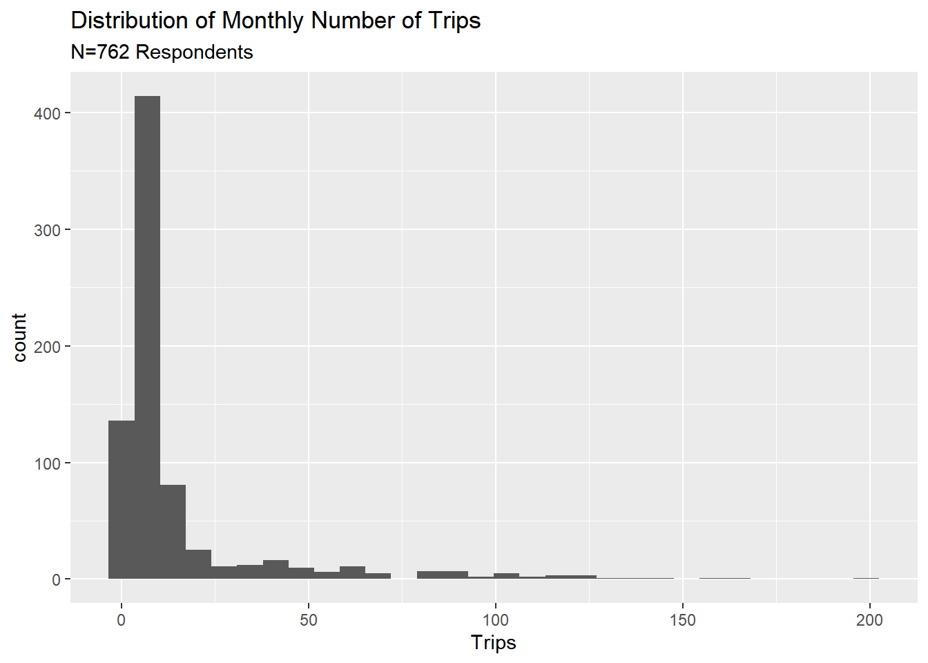
The first sheet contains some basic information about the survey, the second contains the actual survey response data, while the third sheet contains the data dictionary. The trip distribution is quite skewed with most respondents taking very few trips (note: the ggplot command is the main plot command in the ggplot library - an extremely powerful visualization package. You will learn all the details about visualization using ggplot in a later module).
If you have an older Excel file (with extension xls), you can read that in the exact same way as above.
Reading JSON files
JSON is short for Java-Script-Object-Notation and was originally developed as a format for formatting and storing data generated online. It is especially useful when handling irregular data where the number of fields varies by record.
Case Study: Food and Drug Administration Data
The Food and Drug Administration (FDA) is a government agency with a number of different responsibilities. Here we will focus on the “F” part, i.e., food. The FDA monitors and records data on food safety including production, retail and consumption. Since the FDA is a government agency - in this case dealing with issues that are not related to national security - it means that YOU as a citizen can access the data the agency collects.
You can find a number of different FDA datasets to download on https://open.fda.gov/downloads/. These are provided as JSON files. Here we focus on the Food files. There are two: One for food events and one for food enforcement. The food event file contains records of individuals who have gotten sick after consuming good. The food enforcement file contains records of specific types of food that has been recalled. Let’s get these data into R:
We can easily read in json files in Python using the json library. Just like the R version, we need to be aware that this json file as two objects (called “meta” and “results”). Here we first read in the file and then create a pandas data frame from the “results” object:
import polars as pl
import json

enforceFDA = json.load(open("data/food-enforcement-0001-of-0001.json"))
df = pl.DataFrame(enforceFDA["results"])
print(df.shape)
(22969, 25)We can easily read in json files in Python using the json library. Just like the R version, we need to be aware that this json file as two objects (called “meta” and “results”). Here we first read in the file and then create a pandas data frame from the “results” object:
import pandas as pd
import json

enforceFDA = json.load(open("data/food-enforcement-0001-of-0001.json"))
df = pd.DataFrame(enforceFDA["results"])
print(df.shape)
(22969, 25)There are different methods to read these files - here we will use the jsonlite package.
library(jsonlite)
enforceFDA <- fromJSON("data/food-enforcement-0001-of-0001.JSON", flatten = TRUE)
## or
enforceFDA <- fromJSON(unzip("data/food-enforcement-0001-of-0001.json.zip"), flatten = TRUE)
eventFDA <- fromJSON(unzip("data/food-event-0001-of-0001.json.zip"), flatten = TRUE)
The fromJSON function returns an R list with two elements: one called meta which contains some information about the data and another called results which is an R data frame with the actual data.
Let’s take a look at the enforcement events. We can see the first records in the data by
library(tidyverse)
glimpse(enforceFDA$results)
Rows: 22,969
Columns: 24
$ status <chr> "Completed", "Completed", "Ongoing", "Ongoi~
$ city <chr> "Merrillville", "Seattle", "Muscatine", "Ma~
$ state <chr> "IN", "WA", "IA", "MA", "NY", "NC", "CA", "~
$ country <chr> "United States", "United States", "United S~
$ classification <chr> "Class I", "Class II", "Class III", "Class ~
$ product_type <chr> "Food", "Food", "Food", "Food", "Food", "Fo~
$ event_id <chr> "90326", "90729", "90449", "90802", "90748"~
$ recalling_firm <chr> "Albanese Confectionery Group, Inc.", "Trip~
$ address_1 <chr> "5441 E Lincoln Hwy", "9130 15th Pl S Ste D~
$ address_2 <chr> "", "", "", "", "", "", "", "", "", "", "",~
$ postal_code <chr> "46410-5947", "98108-5124", "52761-5809", "~
$ voluntary_mandated <chr> "Voluntary: Firm initiated", "Voluntary: Fi~
$ initial_firm_notification <chr> "Letter", "Two or more of the following: Em~
$ distribution_pattern <chr> "Nationwide", "Distributed in Idaho, Montan~
$ recall_number <chr> "F-1321-2022", "F-1687-2022", "F-1688-2022"~
$ product_description <chr> "Rich s Milk Chocolate Giant Layered Peanut~
$ product_quantity <chr> "18470 pounds", "4438 containers", "14 case~
$ reason_for_recall <chr> "Salmonella. Product made using recalled J~
$ recall_initiation_date <chr> "20220526", "20220808", "20220609", "202208~
$ center_classification_date <chr> "20220621", "20220906", "20220906", "202209~
$ report_date <chr> "20220629", "20220914", "20220914", "202209~
$ code_info <chr> "Mini: 1316 1319 1320 1321 1322 1323 1327 1~
$ more_code_info <chr> "", NA, NA, NA, NA, NA, NA, NA, NA, NA, NA,~
$ termination_date <chr> NA, NA, NA, NA, NA, NA, NA, NA, NA, NA, NA,~So there is a total of 22969 records in the this data with 24 fields. Let’s see what the first recalled product was:
enforceFDA$results$product_description[1][1] "Rich s Milk Chocolate Giant Layered Peanut Butter and Cups Rich s Milk Chocolate Mini Peanut Butter Cups; 2ct 5lb bulk per 10 lb case. Product not retail packaged, distributed for bulk sale at retail."enforceFDA$results$reason_for_recall[1][1] "Salmonella. Product made using recalled Jif peanut butter"enforceFDA$results$recalling_firm[1][1] "Albanese Confectionery Group, Inc."Which company had the most product recalls enforced by the FDA? We can easily get this by counting up the recalling_firm field:
RecallFirmCounts <- table(enforceFDA$results$recalling_firm)
sort(RecallFirmCounts, decreasing = T)[1:10]
     Garden-Fresh Foods, Inc.          Newly Weds Foods Inc
                          633                           438
             Good Herbs, Inc. C & S Wholesale Grocers, Inc.
                          353                           330
           Whole Foods Market    Blue Bell Creameries, L.P.
                          313                           293
     Reser's Fine Foods, Inc.         Sunland, Incorporated
                          221                           219
    Dole Fresh Vegetables Inc            Target Corporation
                          207                           199
Ok - so Garden-Fresh Foods had 633 recall events. This was a simple counting exercise. Later on we will look at much more sophisticated methods for summarizing a database.
Special Use Case: Reading all files in a folder

Here’s a very common situation: You have a large number of files (csv, json or some other format) and you want to read ALL of them into memory. You can do this in a number of different ways but the by far most elegant (and quickest) method is to first read all the file names in the data folder and then apply the relevant read function sequentially.
The folder “turnstile” contains 35 csv files. These files contain data on the number of entries and exits for all turnstiles for the New York City subway system. Each file correspond to one weeks worth of data so we have 35 weeks in total (these files can be downloaded from New York City’s transportation agency’s data page here).
The Python version proceeds by using list comprehension to generate a list of all the data and then stack (“concatenate”) them by repeated use of the read_csv function. Note how short the code below is eventhough we are reading a large number of files:
import polars as pl
import os
import glob

# set path to data and grab file names
path = "data/turnstile/"
all_files = glob.glob(os.path.join(path, "*.txt"))

# Read in each file and concatenate
dfs = [pl.read_csv(f) for f in all_files]
concatenated_df = pl.concat(dfs)

# Print number of rows in final data
print(concatenated_df.shape[0])5366774The Python version proceeds by using list comprehension to generate a list of all the data and then stack (“concatenate”) them by repeated use of the read_csv function. Note how short the code below is eventhough we are reading a large number of files:
import pandas as pd
import os
import glob

# set path to data and grab file names
path = "data/turnstile/"
all_files = glob.glob(os.path.join(path, "*.txt"))

# read in each file and concatenate
concatenated_df = pd.concat([pd.read_csv(f) for f in all_files], ignore_index=True)

# print number of rows in final data
print(concatenated_df.shape[0])5366774Here we will use one of the map functions in the purrr library (part of the tidyverse). These functions all apply a function to a series of R objects. In the following we will use the map_dfr function in conjunction with read_csv.
To read in all files, we first collect all the file names and then apply read_csv to each file and then bind all the rows together into one (very big) data frame.
Here’s the code:
library(tidyverse)

## first get list of all files in data folder
data_path <- "data/turnstile/" # path to data files
files <- dir(data_path, pattern = "*.*", full.names = T) # get file names

## now read in all files
allData <- map_dfr(files, read_csv)
In this code chunk all the file names are collected in the files array. We then apply the function read_csv to each of the elements of this array and stack all the resulting data frames on top of each other.