import polars as pl

transactions = pl.read_csv('data/transactions.csv')
products = pl.read_csv('data/products.csv')
stores = pl.read_csv('data/stores.csv')Group Summaries
 Imagine that you are three years old and someone asks you to take a pile of Lego bricks and count the number of bricks of each color. How would you do this?
If you are a smart three year old you would intuitively use the following algorithm: First divide all bricks into separate piles of identical color, i.e., a pile of red bricks, another of green bricks and so on, and then count the number bricks in each pile. Easy.
Now imagine that you are a 25 year old analyst and your manager asks you to take the company customer database and compute average transaction size per customer for the most recent quarter. This is essentially the Lego problem and you should solve it the same way: First divide transactions into “customer piles” and then compute the average of each pile. This idea of taking a collection of objects and first sorting them and then performing some operation is also the foundation of many modern large scale computing frameworks such as MapReduce.
Grouped Data Summaries in Business Analytics
Whenever you are faced with an objective like the ones above, you should think: Python and the pandas library or R and the tidyverse library. These are packages for performing group operations (and many other things of course). Once you understand how to do this, it will change your life as a data scientist and - quite possibly - permanently make you are a happier person. Seriously.
The basic structure of a group statement is
1.Take some data 2.Define the group assignments for the data 3.Perform some operation on each group
Let us try this out on some real data. As always, you can code and data here: https://www.dropbox.com/scl/fo/pu6pe4i7mncytqbm58q1b/h?rlkey=khuypes7iohteya2d8mfiq0ge&dl=0
Case Study: Retail Transactions
Let’s start out by looking at the same transaction data we used in the relation data module here. We will see how a variety of interesting data summaries easily can be carried out using group-by statements.
Let’s start with a simple objective: What is the total sales (in dollars) for each product (UPC) in the data? Recall that this data is transactions of different products for different stores in different weeks. The current objective requires us to group the data (i.e., rows of the data file) into buckets defined by UPC. For each of the UPC-buckets, we then simply sum the sales (SPEND) to get at the required metric.
We start by importing the polars library and reading in the data:
We can then use the groupby function in pandas to group rows by UPC and then sum sales within all rows for the same UPC:
salesUPC = transactions.groupby('UPC').agg(pl.sum('SPEND'))We group by UPC and sum over SPEND. You can read this - left to right - like you read a recipe for cooking: First take the transactions dataframe, then group it by UPC and then sum the variable SPEND within each group. The reset_index() function at the end of the chain is to make sure that the result is a new pandas dataframe - without that we would get a pandas series. This is fine but dataframes are easier to use for later queries, e.g., merges. The result is a dataframe with one row per UPC:
print(salesUPC.head())shape: (5, 2)
┌─────────────┬───────────┐
│ UPC ┆ SPEND │
│ --- ┆ --- │
│ i64 ┆ f64 │
╞═════════════╪═══════════╡
│ 1111038078 ┆ 113465.39 │
│ 7110410455 ┆ 73248.74 │
│ 31254742735 ┆ 296693.48 │
│ 88491201426 ┆ 954418.23 │
│ 1111009507 ┆ 346753.8 │
└─────────────┴───────────┘Note that the result is sorted by UPC by default. Suppose you wanted the result returned arranged by total SPEND instead. That’s easy - we can just add to the “recipe”:
salesUPC = transactions.groupby('UPC').agg(pl.sum('SPEND')).sort('SPEND', descending=True)Ok - now let’s find the 5 weeks with the highest sales (across all stores and products). In this case we just change the grouping variable to WEEK_END_DATE and then grab the top 5 rows in the sorted dataframe:
salesWeek = transactions.groupby('WEEK_END_DATE').agg(pl.sum('SPEND'))
top5salesWeek = salesWeek.sort('SPEND', descending=True).head(5)
print(top5salesWeek)
shape: (5, 2)
┌───────────────┬───────────┐
│ WEEK_END_DATE ┆ SPEND │
│ --- ┆ --- │
│ str ┆ f64 │
╞═══════════════╪═══════════╡
│ 13-Jan-10 ┆ 261133.84 │
│ 6-Jan-10 ┆ 254203.56 │
│ 9-Feb-11 ┆ 245929.22 │
│ 3-Mar-10 ┆ 235027.24 │
│ 9-Dec-09 ┆ 233886.03 │
└───────────────┴───────────┘Rather than look at UPCs or weeks, now let’s assume that we wanted to find the total sales for each of the four product categories (SNACKS, CEREAL, PIZZA and ORAL HYGIENE). Since each UPCs product information is only found in the product data file, we first merge that with the transactions file and then group by CATEGORY:
transactionsProducts = transactions.join(products, on='UPC')
salesCategory = transactionsProducts.groupby('CATEGORY').agg(pl.sum('SPEND'))
print(salesCategory)
shape: (4, 2)
┌───────────────────────┬──────────┐
│ CATEGORY ┆ SPEND │
│ --- ┆ --- │
│ str ┆ f64 │
╞═══════════════════════╪══════════╡
│ ORAL HYGIENE PRODUCTS ┆ 1.7278e6 │
│ FROZEN PIZZA ┆ 6.4596e6 │
│ BAG SNACKS ┆ 4.7320e6 │
│ COLD CEREAL ┆ 1.5008e7 │
└───────────────────────┴──────────┘We can easily generalize the group-by approach to multiple groups. For example, what is total sales by category for each store? To meet this objective, we must first merge in the product file (to get category information), then group by both STORE_NUM and CATEGORY:
salesCategoryStore = transactionsProducts.groupby(['CATEGORY','STORE_NUM']).agg(pl.sum('SPEND'))
print(salesCategoryStore.head())
shape: (5, 3)
┌───────────────────────┬───────────┬──────────┐
│ CATEGORY ┆ STORE_NUM ┆ SPEND │
│ --- ┆ --- ┆ --- │
│ str ┆ i64 ┆ f64 │
╞═══════════════════════╪═══════════╪══════════╡
│ BAG SNACKS ┆ 23055 ┆ 7730.19 │
│ COLD CEREAL ┆ 2541 ┆ 82259.67 │
│ ORAL HYGIENE PRODUCTS ┆ 17615 ┆ 23234.34 │
│ BAG SNACKS ┆ 23061 ┆ 88277.23 │
│ BAG SNACKS ┆ 29159 ┆ 46111.67 │
└───────────────────────┴───────────┴──────────┘Finally, remember that we can keep adding steps in the chain of operations. For example, we might want the result above in wide format. In this case, we can just add a final pivot_table step at the end:
salesCategoryStoreWide = salesCategoryStore.pivot(values = 'SPEND', index = 'STORE_NUM',columns = 'CATEGORY')<string>:1: DeprecationWarning: In a future version of polars, the default `aggregate_function` will change from `'first'` to `None`. Please pass `'first'` to keep the current behaviour, or `None` to accept the new one.print(salesCategoryStoreWide.head())shape: (5, 5)
┌───────────┬────────────┬─────────────┬───────────────────────┬──────────────┐
│ STORE_NUM ┆ BAG SNACKS ┆ COLD CEREAL ┆ ORAL HYGIENE PRODUCTS ┆ FROZEN PIZZA │
│ --- ┆ --- ┆ --- ┆ --- ┆ --- │
│ i64 ┆ f64 ┆ f64 ┆ f64 ┆ f64 │
╞═══════════╪════════════╪═════════════╪═══════════════════════╪══════════════╡
│ 23055 ┆ 7730.19 ┆ 84935.97 ┆ 7730.11 ┆ 42152.96 │
│ 2541 ┆ 16084.14 ┆ 82259.67 ┆ 11965.54 ┆ 34656.53 │
│ 17615 ┆ 28017.43 ┆ 139788.43 ┆ 23234.34 ┆ 65096.92 │
│ 23061 ┆ 88277.23 ┆ 208878.41 ┆ 19951.5 ┆ 98472.77 │
│ 29159 ┆ 46111.67 ┆ 167652.55 ┆ 19101.84 ┆ 60915.59 │
└───────────┴────────────┴─────────────┴───────────────────────┴──────────────┘Let’s start with a simple objective: What is the total sales (in dollars) for each product (UPC) in the data? Recall that this data is transactions of different products for different stores in different weeks. The current objective requires us to group the data (i.e., rows of the data file) into buckets defined by UPC. For each of the UPC-buckets, we then simply sum the sales (SPEND) to get at the required metric.
We start by importing the pandas library and reading in the data:
import pandas as pd

transactions = pd.read_csv('data/transactions.csv')
products = pd.read_csv('data/products.csv')
stores  = pd.read_csv('data/stores.csv')
We can then use the groupby function in pandas to group rows by UPC and then sum sales within all rows for the same UPC:
salesUPC = transactions.groupby(['UPC'])['SPEND'].sum().reset_index()We group by UPC and sum over SPEND. You can read this - left to right - like you read a recipe for cooking: First take the transactions dataframe, then group it by UPC and then sum the variable SPEND within each group. The reset_index() function at the end of the chain is to make sure that the result is a new pandas dataframe - without that we would get a pandas series. This is fine but dataframes are easier to use for later queries, e.g., merges. The result is a dataframe with one row per UPC:
print(salesUPC.head()) UPC SPEND
0 1111009477 912633.74
1 1111009497 715124.34
2 1111009507 346753.80
3 1111035398 95513.37
4 1111038078 113465.39Note that the result is sorted by UPC by default. Suppose you wanted the result returned arranged by total SPEND instead. That’s easy - we can just add to the “recipe”:
salesUPC = transactions.groupby(['UPC'])['SPEND'].sum().reset_index().sort_values(by=['SPEND'], ascending = False)Ok - now let’s find the 5 weeks with the highest sales (across all stores and products). In this case we just change the grouping variable to WEEK_END_DATE and then grab the top 5 rows in the sorted dataframe:
salesWeek = transactions.groupby(['WEEK_END_DATE'])['SPEND'].sum().reset_index()
print(salesWeek.sort_values(by=['SPEND'], ascending = False)[0:5])
WEEK_END_DATE SPEND
20 13-Jan-10 261133.84
136 6-Jan-10 254203.56
151 9-Feb-11 245929.22
116 3-Mar-10 235027.24
150 9-Dec-09 233886.03Rather than look at UPCs or weeks, now let’s assume that we wanted to find the total sales for each of the four product categories (SNACKS, CEREAL, PIZZA and ORAL HYGIENE). Since each UPCs product information is only found in the product data file, we first merge that with the transactions file and then group by CATEGORY:
transactionsProducts = transactions.merge(products, on = 'UPC')
salesCategory = transactionsProducts.groupby(['CATEGORY'])['SPEND'].sum()
print(salesCategory)
CATEGORY
BAG SNACKS 4731982.53
COLD CEREAL 15008351.27
FROZEN PIZZA 6459557.59
ORAL HYGIENE PRODUCTS 1727831.19
Name: SPEND, dtype: float64We can easily generalize the group-by approach to multiple groups. For example, what is total sales by category for each store? To meet this objective, we must first merge in the product file (to get category information), then group by both STORE_NUM and CATEGORY:
salesCategoryStore = transactionsProducts.groupby(['CATEGORY','STORE_NUM'])['SPEND'].sum().reset_index()
print(salesCategoryStore.head())
CATEGORY STORE_NUM SPEND
0 BAG SNACKS 367 20988.36
1 BAG SNACKS 387 100710.62
2 BAG SNACKS 389 137481.40
3 BAG SNACKS 613 61620.43
4 BAG SNACKS 623 32654.77Finally, remember that we can keep adding steps in the chain of operations. For example, we might want the result above in wide format. In this case, we can just add a final pivot_table step at the end:
salesCategoryStoreWide = pd.pivot_table(salesCategoryStore,index='STORE_NUM',columns='CATEGORY',values='SPEND').reset_index()
print(salesCategoryStoreWide.head())
CATEGORY STORE_NUM BAG SNACKS ... FROZEN PIZZA ORAL HYGIENE PRODUCTS
0 367 20988.36 ... 52475.44 6871.20
1 387 100710.62 ... 102733.14 34575.06
2 389 137481.40 ... 116476.88 29707.91
3 613 61620.43 ... 89158.54 23485.61
4 623 32654.77 ... 87677.56 24244.83
[5 rows x 5 columns]Suppose that you want to calculate multiple summaries in one groupby statement. We can solve this by creating a function that calculates any summary on each groupby subset of the data and then apply that function to each of those subsets. Here’s an example:
# Find total spend, average spend, minimum spend, maximum spend across all weeks for each
# store and category

# this function contains all the summaries we want for each of the groupby combinations
def f(x):
    d = {}
    d['totalSpend'] = x['SPEND'].sum()
    d['avgSpend'] = x['SPEND'].sum()
    d['minSpend'] = x['SPEND'].min()
    d['maxSpend'] = x['SPEND'].max()
    return pd.Series(d)

salesCategoryStoreStats = transactionsProducts.groupby(['CATEGORY','STORE_NUM']).apply(f)

print(salesCategoryStoreStats.head())
totalSpend avgSpend minSpend maxSpend
CATEGORY STORE_NUM
BAG SNACKS 367 20988.36 20988.36 0.00 106.64
387 100710.62 100710.62 2.50 268.95
389 137481.40 137481.40 2.00 305.14
613 61620.43 61620.43 2.39 150.80
623 32654.77 32654.77 1.12 107.06Let’s start with a simple objective: What is the total sales (in dollars) for each product (UPC) in the data? Recall that this data is transactions of different products for different stores in different weeks. The current objective requires us to group the data (i.e., rows of the data file) into buckets defined by UPC. For each of the UPC-buckets, we then simply sum the sales (SPEND) to get at the required metric.
We start by loading the required packaged and the data:
library(tidyverse)

transactions <- read_csv('/data/transactions.csv')
products <- read_csv('data/products.csv')
stores <- read_csv('data/stores.csv')
Warning: package 'tidyverse' was built under R version 4.1.3Warning: package 'ggplot2' was built under R version 4.1.3Warning: package 'tibble' was built under R version 4.1.3Warning: package 'stringr' was built under R version 4.1.3Warning: package 'forcats' was built under R version 4.1.3-- Attaching core tidyverse packages ------------------------ tidyverse 2.0.0 --
v dplyr 1.1.1.9000 v readr 2.0.2
v forcats 1.0.0 v stringr 1.5.0
v ggplot2 3.4.2 v tibble 3.2.1
v lubridate 1.8.0 v tidyr 1.1.4
v purrr 0.3.4
-- Conflicts ------------------------------------------ tidyverse_conflicts() --
x dplyr::filter() masks stats::filter()
x dplyr::lag() masks stats::lag()
i Use the conflicted package (<http://conflicted.r-lib.org/>) to force all conflicts to become errors
Rows: 524950 Columns: 12
-- Column specification --------------------------------------------------------
Delimiter: ","
chr (1): WEEK_END_DATE
dbl (11): STORE_NUM, UPC, UNITS, VISITS, HHS, SPEND, PRICE, BASE_PRICE, FEAT...
i Use `spec()` to retrieve the full column specification for this data.
i Specify the column types or set `show_col_types = FALSE` to quiet this message.
Rows: 58 Columns: 6
-- Column specification --------------------------------------------------------
Delimiter: ","
chr (5): DESCRIPTION, MANUFACTURER, CATEGORY, SUB_CATEGORY, PRODUCT_SIZE
dbl (1): UPC
i Use `spec()` to retrieve the full column specification for this data.
i Specify the column types or set `show_col_types = FALSE` to quiet this message.
Rows: 77 Columns: 9
-- Column specification --------------------------------------------------------
Delimiter: ","
chr (4): STORE_NAME, ADDRESS_CITY_NAME, ADDRESS_STATE_PROV_CODE, SEG_VALUE_NAME
dbl (5): STORE_ID, MSA_CODE, PARKING_SPACE_QTY, SALES_AREA_SIZE_NUM, AVG_WEE...
i Use `spec()` to retrieve the full column specification for this data.
i Specify the column types or set `show_col_types = FALSE` to quiet this message.What is the total sales (in dollars) for each product (UPC) in the data? Recall that this data is transactions of different products for different stores in different weeks. The current objective requires us to group the data (i.e., rows of the data file) into buckets defined by UPC. For each of the UPC-buckets, we then simply sum the sales (SPEND) to get at the required metric:
salesUPC <- transactions %>%
  group_by(UPC) %>%
  summarize(total = sum(SPEND))
We group by UPC and sum over SPEND. You can read this like you read a recipe for cooking. Think of the %> sign as an “and”: First take the transactions dataframe AND then group it by UPC AND sum the variable SPEND within each group. The result is a dataframe with one row per UPC:
head(salesUPC)# A tibble: 6 x 2
UPC total
<dbl> <dbl>
1 1111009477 912634.
2 1111009497 715124.
3 1111009507 346754.
4 1111035398 95513.
5 1111038078 113465.
6 1111038080 88450.Note that we can easily add more steps to the “recipe” above - for example - add information on the UPCs and sort in descinding order of spending:
salesUPCsort <- salesUPC %>%
  inner_join(products, by = 'UPC') %>%
  arrange(desc(total))

head(salesUPCsort)
# A tibble: 6 x 7
UPC total DESCRIPTION MANUFACTURER CATEGORY SUB_CATEGORY PRODUCT_SIZE
<dbl> <dbl> <chr> <chr> <chr> <chr> <chr>
1 1600027527 2.05e6 GM HONEY N~ GENERAL MI COLD CE~ ALL FAMILY ~ 12.25 OZ
2 3800031838 1.48e6 KELL FROST~ KELLOGG COLD CE~ KIDS CEREAL 15 OZ
3 7192100339 1.44e6 DIGRN PEPP~ TOMBSTONE FROZEN ~ PIZZA/PREMI~ 28.3 OZ
4 1600027528 1.43e6 GM CHEERIOS GENERAL MI COLD CE~ ALL FAMILY ~ 18 OZ
5 1600027564 1.38e6 GM CHEERIOS GENERAL MI COLD CE~ ALL FAMILY ~ 12 OZ
6 3800031829 1.22e6 KELL BITE ~ KELLOGG COLD CE~ ALL FAMILY ~ 18 OZ Suppose we wanted to identify the 5 weeks with the highest total weekly spending across all stores and products. Easy - we just group by the week variable WEEK_END_DATA and pick out the top 5:
salesWeek <- transactions %>%
  group_by(WEEK_END_DATE ) %>%
  summarize(total = sum(SPEND)) %>%
  top_n(5,wt = total)

salesWeek
# A tibble: 5 x 2
WEEK_END_DATE total
<chr> <dbl>
1 13-Jan-10 261134.
2 3-Mar-10 235027.
3 6-Jan-10 254204.
4 9-Dec-09 233886.
5 9-Feb-11 245929.Rather than look at UPCs or weeks, now let’s assume that we wanted to find the total sales for each of the four product categories (SNACKS, CEREAL, PIZZA and ORAL HYGIENE). Since each UPCs product information is only found in the product data file, we first join that with the transactions file and then group by CATEGORY:
transactionsProduct <- transactions %>%
  inner_join(products, by = 'UPC')

salesCategory <- transactionsProduct %>%
  group_by(CATEGORY) %>%
  summarize(total = sum(SPEND))

salesCategory
# A tibble: 4 x 2
CATEGORY total
<chr> <dbl>
1 BAG SNACKS 4731983.
2 COLD CEREAL 15008351.
3 FROZEN PIZZA 6459558.
4 ORAL HYGIENE PRODUCTS 1727831.We can easily generalize the group-by approach to multiple groups. For example, what is total sales by category for each store? To meet this objective, we must first join the product file (to get category information), then group by both STORE_NUM and CATEGORY:
salesCategoryStore <- transactionsProduct %>%
  group_by(STORE_NUM,CATEGORY) %>%
  summarize(total = sum(SPEND))
`summarise()` has grouped output by 'STORE_NUM'. You can override using the
`.groups` argument.head(salesCategoryStore)# A tibble: 6 x 3
# Groups: STORE_NUM [2]
STORE_NUM CATEGORY total
<dbl> <chr> <dbl>
1 367 BAG SNACKS 20988.
2 367 COLD CEREAL 127585.
3 367 FROZEN PIZZA 52475.
4 367 ORAL HYGIENE PRODUCTS 6871.
5 387 BAG SNACKS 100711.
6 387 COLD CEREAL 241718.Finally, remember that we can keep adding steps in the chain (by adding more lines with %>%). For example, we might want to wide format of result above. In this case, we can just add a final pivot_wider step at the end:
salesCategoryStore <- transactionsProduct %>%
  group_by(STORE_NUM,CATEGORY) %>%
  summarize(total = sum(SPEND)) %>%
  pivot_wider(id_cols = 'STORE_NUM',names_from = 'CATEGORY',values_from = 'total')
`summarise()` has grouped output by 'STORE_NUM'. You can override using the
`.groups` argument.head(salesCategoryStore)# A tibble: 6 x 5
# Groups: STORE_NUM [6]
STORE_NUM `BAG SNACKS` `COLD CEREAL` `FROZEN PIZZA` `ORAL HYGIENE PRODUCTS`
<dbl> <dbl> <dbl> <dbl> <dbl>
1 367 20988. 127585. 52475. 6871.
2 387 100711. 241718. 102733. 34575.
3 389 137481. 327986. 116477. 29708.
4 613 61620. 207302. 89159. 23486.
5 623 32655. 165673. 87678. 24245.
6 2277 235623. 480789. 190066. 66659.Suppose that you want to calculate multiple summaries in one groupby statement. Easy - you just keep adding more statements in the summarize function:
##
## Find total spend, average spend, minimum spend, maximum spend across all weeks for each
## store and category
##
salesCategoryStoreStats <- transactions %>%
  inner_join(products, by = 'UPC') %>%
  group_by(STORE_NUM,CATEGORY) %>%
  summarize(totalSpend = sum(SPEND),
            avgSpend = mean(SPEND),
            minSpend = min(SPEND),
            maxSpend = max(SPEND))
`summarise()` has grouped output by 'STORE_NUM'. You can override using the
`.groups` argument.head(salesCategoryStoreStats)# A tibble: 6 x 6
# Groups: STORE_NUM [2]
STORE_NUM CATEGORY totalSpend avgSpend minSpend maxSpend
<dbl> <chr> <dbl> <dbl> <dbl> <dbl>
1 367 BAG SNACKS 20988. 15.2 0 107.
2 367 COLD CEREAL 127585. 58.2 1.65 492.
3 367 FROZEN PIZZA 52475. 39.2 3.89 250.
4 367 ORAL HYGIENE PRODUCTS 6871. 6.63 1 39.9
5 387 BAG SNACKS 100711. 54.5 2.5 269.
6 387 COLD CEREAL 241718. 130. 1.99 796. Case Study: Pandemic Library Checkouts
 The city of Seattle’s open data portal contains a database that records the monthly checkout count of every item (mostly books) in the Seattle Public Library system. You can find the full data here.
Let’s do a quick analysis of how the global Covid-19 pandemic impacted usage of the public library system in Seattle. Here we use only data for the years 2019-2021. Did users check out more or fewer books during the pandemic compared to before? Which books were more popular during the lockdown than before? This and many other interesting questions can be answered using this database.
Since seaborn does not directly support Polars Data Frame we will stick to Pandas
We start by loading the required libraries and data and print the column names:
import pandas as pd

checkouts = pd.read_csv('data/Checkouts_by_Title.csv')
for col in checkouts.columns:
    print(col)
<string>:1: DtypeWarning: Columns (7) have mixed types. Specify dtype option on import or set low_memory=False.UsageClass
CheckoutType
MaterialType
CheckoutYear
CheckoutMonth
Checkouts
Title
ISBN
Creator
Subjects
Publisher
PublicationYear
yearEach row in the data is a (item,year,month) combination and the column Checkouts tells us how many times the corresponding item was checked out in year CheckoutYear and month CheckoutMonth.
Let’s start by looking at total checkouts by year and month. We use a group-by to get monthly totals and the plot them to inspect the trends:
import seaborn as sns
totalYearMonth = checkouts.groupby(['CheckoutYear','CheckoutMonth'])['Checkouts'].sum().reset_index()
totalYearMonth['CheckoutYear'] = totalYearMonth.CheckoutYear.astype('category')

sns.lineplot(x="CheckoutMonth", y="Checkouts",
             hue="CheckoutYear",
             data=totalYearMonth)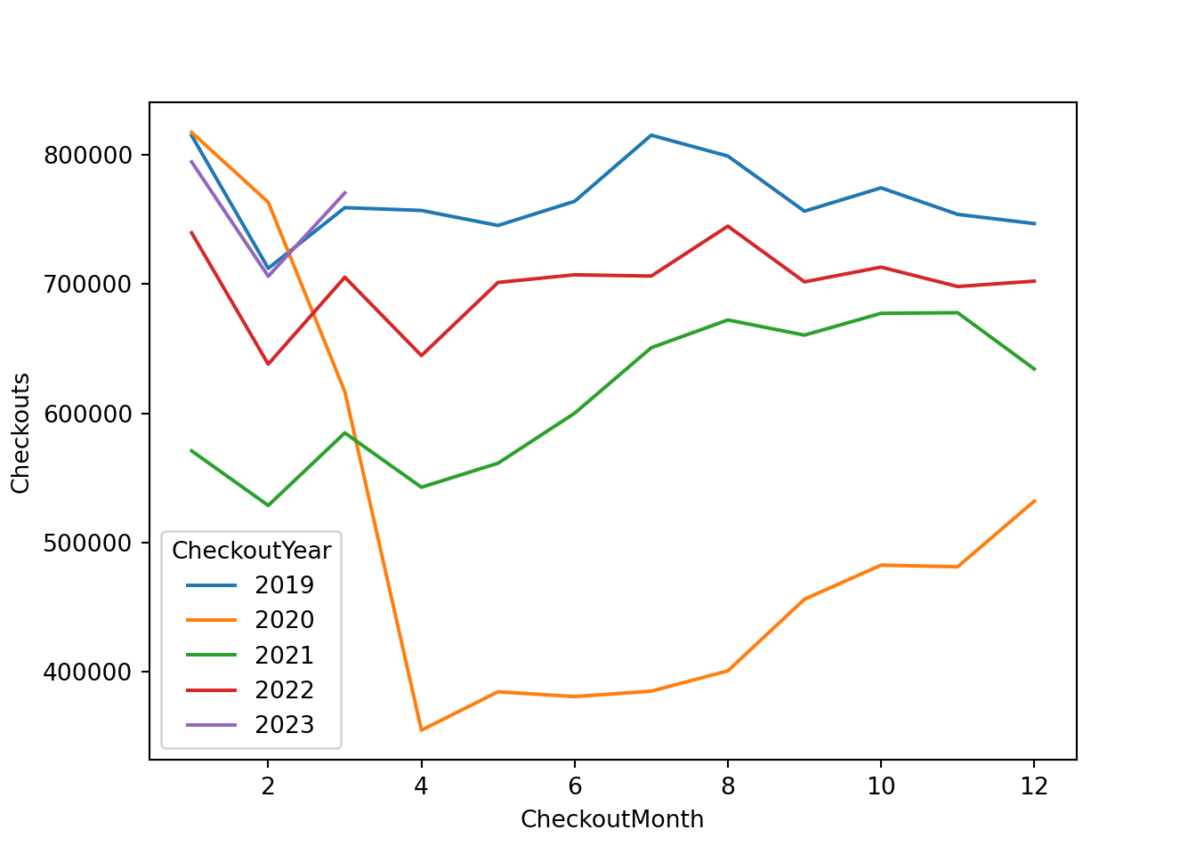
We see a massive drop in checkouts starting in month 3 and 4 of 2020. This is consistent with the national Covid-19 emergency that was declared in mid-March 2020. Around this time many states in the US went into lockdown with businesses closing and most people working from home. In fact the Seattle Public libaries themselves were closed for a large part of 2020. Therefore it was impossible to checkout physical books from the library during this time. This explains the large drop in checkouts in early 2020.
While the libraries were closed, people could still check out digital items online. To see what these patterns look like we can focus attention on ebooks:
checkoutsE = checkouts[checkouts['MaterialType'] == 'EBOOK']

totalYearMonth = checkoutsE.groupby(['CheckoutYear','CheckoutMonth'])['Checkouts'].sum().reset_index()
totalYearMonth['CheckoutYear'] = totalYearMonth.CheckoutYear.astype('category')

sns.lineplot(x="CheckoutMonth", y="Checkouts",
             hue="CheckoutYear",
             data=totalYearMonth)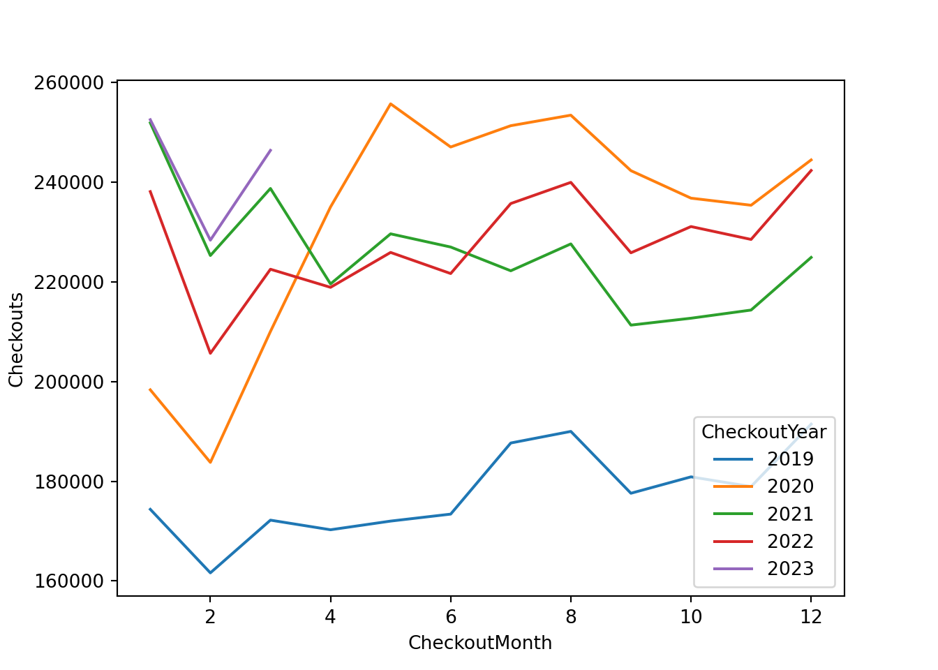
Ok - this is interesting: We now see a large INCREASE in checkouts starting around the beginning of the lockdown. One possible explanation is simply people having more time on their hands (while working from home).
Did all types of ebook checkouts increase by the same amount or did some increase and others decrease? To answer this we can look at each book’s subject (Subjects). There are a LOT of different book subjects in the data - here we focus attention on the top 25 most frequent subjects in the data:
n = 25
topSubjects = checkoutsE['Subjects'].value_counts()[:n].index.tolist()
print(topSubjects)
['Fiction, Literature', 'Fiction, Mystery', 'Juvenile Fiction, Juvenile Literature', 'Fiction, Romance', 'Cooking & Food, Nonfiction', 'Fiction, Mystery, Suspense, Thriller', 'Fantasy, Fiction', 'Fiction, Literature, Romance', 'Fiction, Historical Fiction, Romance', 'Fantasy, Fiction, Romance', 'Fiction, Science Fiction', 'Juvenile Fiction, Picture Book Fiction', 'Fiction, Suspense, Thriller', 'Fiction, Romance, Historical Fiction', 'Fiction, Mystery, Thriller', 'Fiction, Thriller', 'Fantasy, Juvenile Fiction, Juvenile Literature', 'Business, Nonfiction', 'Health & Fitness, Nonfiction', 'History, Nonfiction', 'Fiction, Literature, Historical Fiction', 'Fiction, Literature, Mystery', 'Juvenile Fiction, Juvenile Literature, Picture Book Fiction', 'Fiction, Literature, Suspense, Thriller', 'Biography & Autobiography, Nonfiction']Since the overall level of checkouts of ebooks is increasing, we can look at the relative share of each subject and then study which subjects have increasing versus decreasing shares during the lockdown period. So we will filter out the relevant subjects, then do a three-level group-by to get total checkout counts at the (Year,Month,Subject) level and then divide by the total to get shares:
checkoutsEsub = checkoutsE[checkoutsE.Subjects.isin(topSubjects)]

totalYearMonth = totalYearMonth.rename(columns={'Checkouts':'Total'})
totalSubjectYearMonth = checkoutsEsub.groupby(['CheckoutYear','CheckoutMonth','Subjects'])['Checkouts'].sum().reset_index()
totalSubjectYearMonth = totalSubjectYearMonth.merge(totalYearMonth, on = ['CheckoutYear','CheckoutMonth'])
totalSubjectYearMonth['Share'] = totalSubjectYearMonth['Checkouts']/totalSubjectYearMonth['Total']
We drop the 2021 data, convert the year to a category to get correct colors on the visualization and the plot shares for each subject:
totalSubjectYearMonth19_20 = totalSubjectYearMonth[totalSubjectYearMonth['CheckoutYear'] != 2021]
totalSubjectYearMonth19_20.loc[:,"CheckoutYear"] = totalSubjectYearMonth19_20.loc[:,'CheckoutYear'].astype('category')

g = sns.FacetGrid(totalSubjectYearMonth19_20, hue="CheckoutYear", col="Subjects",sharey=False,col_wrap=3,height=4.5, aspect=1)
g = g.map(sns.lineplot, "CheckoutMonth", "Share")
g.add_legend()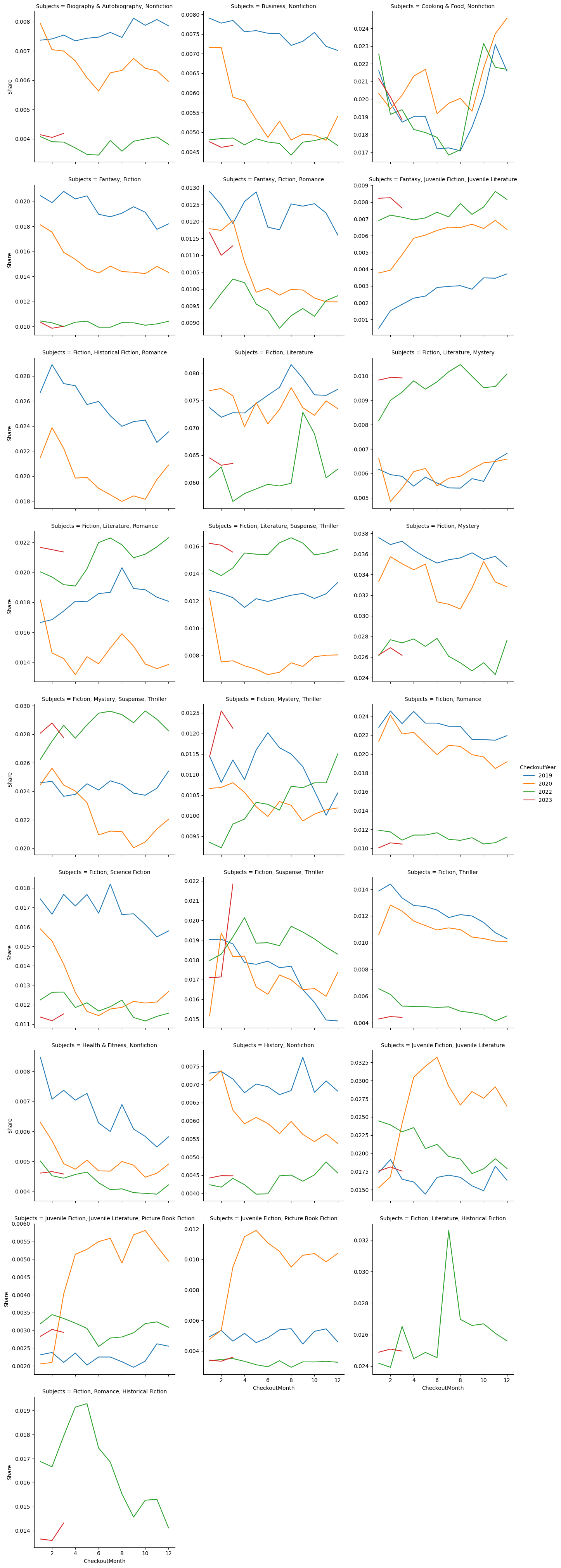
These shares are quite informative. In relative terms it is clear that checkouts of ebooks for children is the main driver of the increase in overall ebook checkouts.
We start by loading the required libraries and data and then taking a peek at the data:
library(tidyverse)
checkouts <- read_csv('data/Checkouts_by_Title.csv')
head(checkouts)
Rows: 9750667 Columns: 13
-- Column specification --------------------------------------------------------
Delimiter: ","
chr (9): UsageClass, CheckoutType, MaterialType, Title, ISBN, Creator, Subje...
dbl (4): CheckoutYear, CheckoutMonth, Checkouts, year
i Use `spec()` to retrieve the full column specification for this data.
i Specify the column types or set `show_col_types = FALSE` to quiet this message.# A tibble: 6 x 13
UsageClass CheckoutType MaterialType CheckoutYear CheckoutMonth Checkouts
<chr> <chr> <chr> <dbl> <dbl> <dbl>
1 Digital OverDrive EBOOK 2019 1 1
2 Digital OverDrive EBOOK 2019 2 1
3 Digital OverDrive EBOOK 2019 2 2
4 Digital OverDrive EBOOK 2019 3 2
5 Physical Horizon VIDEODISC 2019 3 2
6 Digital OverDrive EBOOK 2019 3 2
# i 7 more variables: Title <chr>, ISBN <chr>, Creator <chr>, Subjects <chr>,
# Publisher <chr>, PublicationYear <chr>, year <dbl>Each row in the data is a (item,year,month) combination and the column Checkouts tells us how many times the corresponding item was checked out in year CheckoutYear and month CheckoutMonth.
Let’s start by looking at total checkouts by year and month. We use a group-by to get monthly totals and the plot them to inspect the trends:
totalYearMonth <- checkouts %>%
  group_by(CheckoutYear,CheckoutMonth) %>%
  summarize(total = sum(Checkouts))
`summarise()` has grouped output by 'CheckoutYear'. You can override using the
`.groups` argument.totalYearMonth %>%
mutate(CheckoutMonth = factor(CheckoutMonth),
CheckoutYear = factor(CheckoutYear)) %>%
ggplot(aes(x = CheckoutMonth, y = total, group = CheckoutYear, color = CheckoutYear)) + geom_line() +
labs(title = 'Checkouts by Year and Month')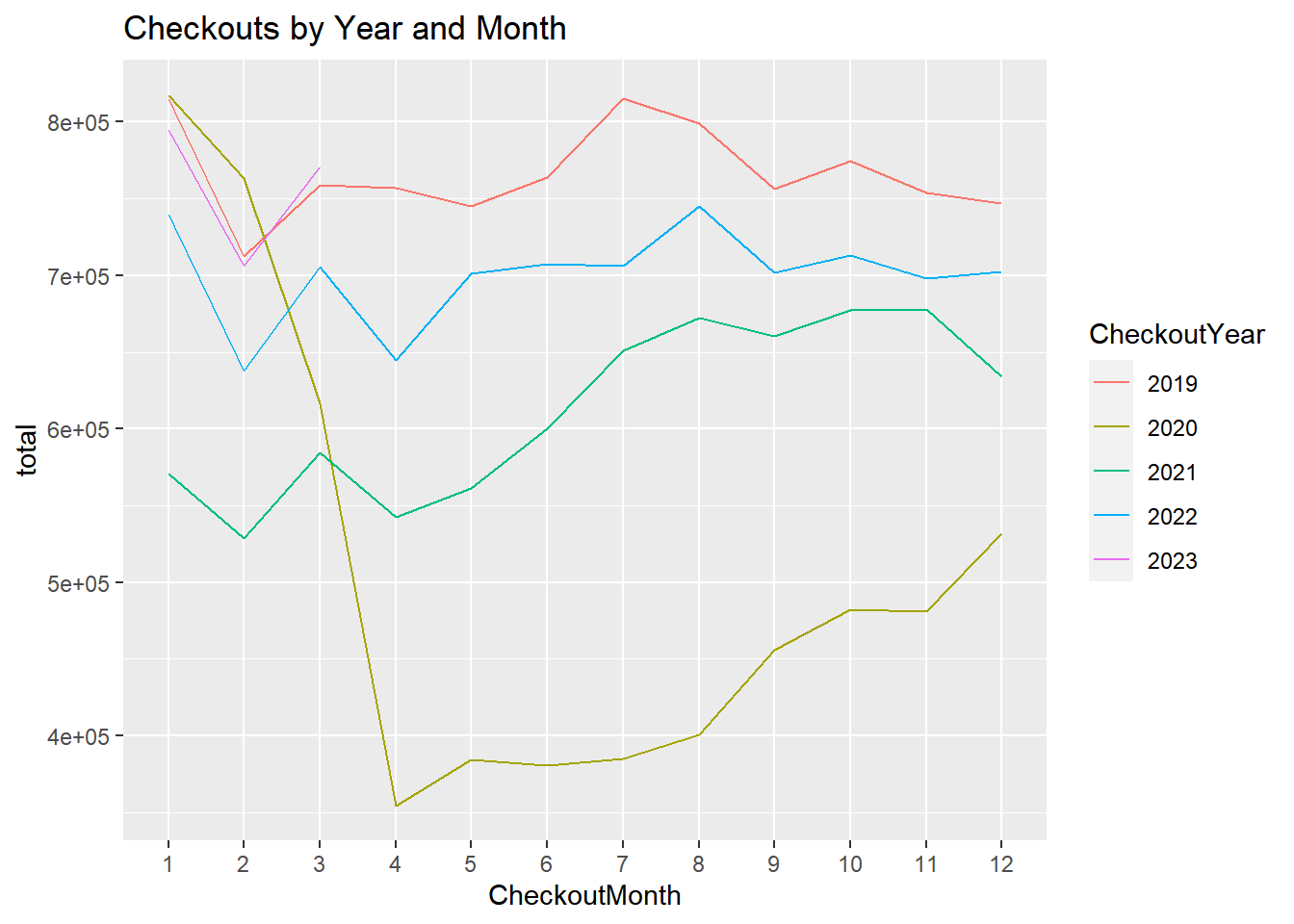
We see a massive drop in checkouts starting in month 3 and 4 of 2020. This is consistent with the national Covid-19 emergency that was declared in mid-March 2020. Around this time many states in the US went into lockdown with businesses closing and most people working from home. In fact the Seattle Public libaries themselves were closed for a large part of 2020. Therefore it was impossible to checkout physical books from the library during this time. This explains the large drop in checkouts in early 2020.
While the libraries were closed, people could still check out digital items online. To see what these patterns look like we can focus attention on ebooks:
checkoutsE <- checkouts %>%
  filter(MaterialType == 'EBOOK')

totalYearMonth <- checkoutsE %>%
  group_by(CheckoutYear,CheckoutMonth) %>%
  summarize(total = sum(Checkouts))
`summarise()` has grouped output by 'CheckoutYear'. You can override using the
`.groups` argument.totalYearMonth %>%
mutate(CheckoutMonth = factor(CheckoutMonth),
CheckoutYear = factor(CheckoutYear)) %>%
ggplot(aes(x = CheckoutMonth, y = total, group = CheckoutYear, color = CheckoutYear)) + geom_line() +
labs(title = 'Checkouts by Year and Month',
subtitle = 'Ebooks Only')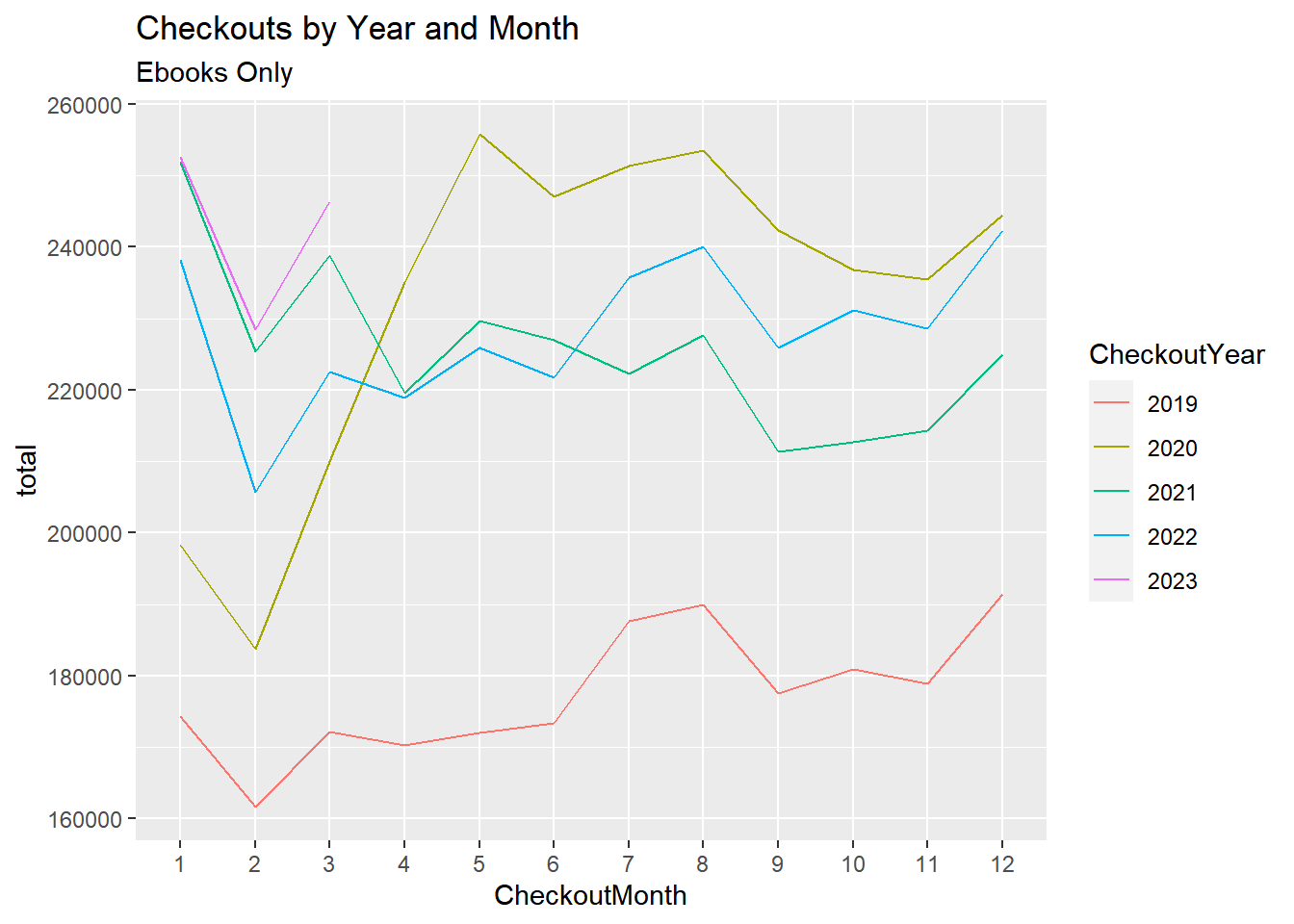
Ok - this is interesting: We now see a large INCREASE in checkouts starting around the beginning of the lockdown. One possible explanation is simply people having more time on their hands (while working from home).
Did all types of ebook checkouts increase by the same amount or did some increase and others decrease? To answer this we can look at each book’s subject (Subjects). There are a LOT of different book subjects in the data - here we focus attention on the top 25 most frequent subjects in the data:
topSubjects <- checkoutsE %>%
  count(Subjects, sort = T) %>%
  slice(1:25)
Since the overall level of checkouts of ebooks is increasing, we can look at the relative share of each subject and then study which subjects have increasing versus decreasing shares during the lockdown period. So we will filter out the relevant subjects, then do a three-level group-by to get total checkout counts at the (Year,Month,Subject) level and then divide by the total to get shares:
totalSubjectYearMonth <- checkoutsE %>%
  filter(Subjects %in% topSubjects$Subjects) %>%
  group_by(CheckoutYear,CheckoutMonth,Subjects) %>%
  summarize(totalSubject = sum(Checkouts)) %>%
  left_join(totalYearMonth, by = c('CheckoutYear','CheckoutMonth')) %>%
  mutate(share = totalSubject/total)
`summarise()` has grouped output by 'CheckoutYear', 'CheckoutMonth'. You can
override using the `.groups` argument.The resulting dataframe has quite a bit of data, so it seems to visualize it in order to inspect all patterns:
totalSubjectYearMonth %>%
  filter(!CheckoutYear==2021) %>%
  mutate(CheckoutMonth = factor(CheckoutMonth),
         CheckoutYear = factor(CheckoutYear)) %>%
  ggplot(aes(x = CheckoutMonth, y = share, group = CheckoutYear, color = CheckoutYear)) + geom_line() +
  scale_y_continuous(labels = scales::percent) +
  labs(title = 'Ebook Subject Checkout Share by Year and Month') +
  facet_wrap(~Subjects,scales='free',ncol = 3)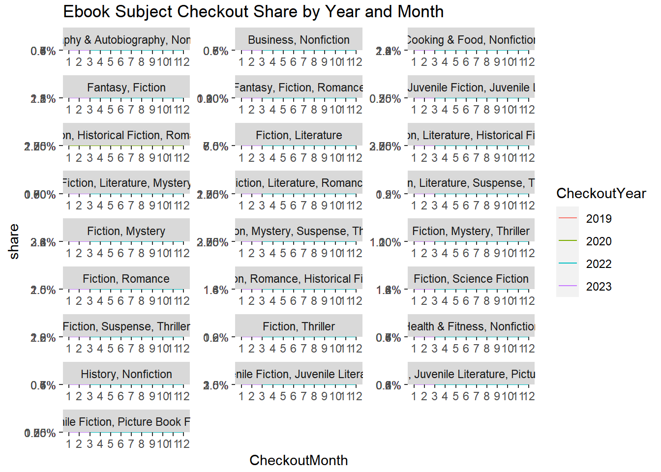
These shares are quite informative. In relative terms it is clear that checkouts of ebooks for children is the main driver of the increase in overall ebook checkouts.
Case Study: Product Related Injuries
 Every year the US federal government collects information on consumer product related injuries and makes the data available in a public database called theNational Electronic Injury Surveillance System (NEISS). The idea is to track consumer products who may be risky to use and prone to creating injuries.
The data is made available as a csv file with an accompanying data dictionary file.
Let’s start by importing these files:
import polars as pl
import numpy as np

neiss19 = pl.read_csv('data/neiss2019.csv')
neiss19f = pl.read_csv('data/neiss2019_format.csv')

for col in neiss19.columns:
    print(col)
CPSC_Case_Number
Treatment_Date
Age
Sex
Race
Other_Race
Hispanic
Body_Part
Diagnosis
Other_Diagnosis
Body_Part_2
Diagnosis_2
Other_Diagnosis_2
Disposition
Location
Fire_Involvement
Product_1
Product_2
Product_3
Alcohol
Drug
Narrative
Stratum
PSU
WeightEach row in the data is one injury with some basic information on the person being injured (age, gender, race), the body part being injured and the type of product involved in the injury (Product_1, Product_2 etc.). Let’s start by finding the most frequent products associated with injuries in the data:
n = 10
topProd = neiss19['Product_1'].value_counts().sort(by="counts", descending=True).limit(n)
topProd = topProd.rename({'Product_1': 'Product_1', 'counts': 'n'})

print(topProd)
shape: (10, 2)
┌───────────┬───────┐
│ Product_1 ┆ n │
│ --- ┆ --- │
│ i64 ┆ u32 │
╞═══════════╪═══════╡
│ 1807 ┆ 29895 │
│ 1842 ┆ 28779 │
│ 4076 ┆ 21043 │
│ 1205 ┆ 12642 │
│ … ┆ … │
│ 4074 ┆ 9129 │
│ 1884 ┆ 7840 │
│ 611 ┆ 7661 │
│ 1893 ┆ 7275 │
└───────────┴───────┘Hmm..ok - this is not very insightful since we don’t know what the product codes are. These are contained in the data dictionary that we imported along with the raw data. The product codes can be found in the rows where the first column Variable is equal to PROD:
neiss19_prod = neiss19f.filter(pl.col('Variable') == 'PROD')

print(neiss19_prod.select(['value', 'label']).head())
shape: (5, 2)
┌──────────────────┬───────────────────────────────────┐
│ value ┆ label │
│ --- ┆ --- │
│ str ┆ str │
╞══════════════════╪═══════════════════════════════════╡
│ 101 ┆ 101 - WASHING MACHINES WITHOUT W… │
│ 102 ┆ 102 - WRINGER WASHING MACHINES │
│ 103 ┆ 103 - WASHING MACHINES WITH UNHE… │
│ 106 ┆ 106 - ELECTRIC CLOTHES DRYERS WI… │
│ 107 ┆ 107 - GAS CLOTHES DRYERS WITHOUT… │
└──────────────────┴───────────────────────────────────┘The column label contains the name of the product category. The formatting is a little annoying since the label also contains the value of the product category (e.g., 101 for the first category). Let’s clean this up a bit: we will extract the substring after the “-” and convert the value column to numeric (since it is a numeric in the raw data and we will need to join the two dataframes):
##prod_labels = neiss19_prod.clone()
neiss19_prod = neiss19_prod.with_columns(['label', pl.col('label').str.split_exact("-", 1).struct.rename_fields(["first_part", "second_part"]).alias("label_1"),]).unnest("label_1")

#neiss19_prod = neiss19_prod.with_columns('value', pl.col('value').cast(pl.Int64)).alias('value_int')

neiss19_prod = neiss19_prod.with_columns([
    pl.col('first_part').cast(pl.Int64,strict=False)
])

print(neiss19_prod[['first_part', 'second_part']].head())
### Throwing Error!
shape: (5, 2)
┌────────────┬───────────────────────────────────┐
│ first_part ┆ second_part │
│ --- ┆ --- │
│ i64 ┆ str │
╞════════════╪═══════════════════════════════════╡
│ null ┆ WASHING MACHINES WITHOUT WRINGE… │
│ null ┆ WRINGER WASHING MACHINES │
│ null ┆ WASHING MACHINES WITH UNHEATED … │
│ null ┆ ELECTRIC CLOTHES DRYERS WITHOUT… │
│ null ┆ GAS CLOTHES DRYERS WITHOUT WASH… │
└────────────┴───────────────────────────────────┘Let’s start by importing these files:
import pandas as pd
import numpy as np

neiss19 = pd.read_csv('data/neiss2019.csv')
neiss19f = pd.read_csv('data/neiss2019_format.csv')

for col in neiss19.columns:
    print(col)
CPSC_Case_Number
Treatment_Date
Age
Sex
Race
Other_Race
Hispanic
Body_Part
Diagnosis
Other_Diagnosis
Body_Part_2
Diagnosis_2
Other_Diagnosis_2
Disposition
Location
Fire_Involvement
Product_1
Product_2
Product_3
Alcohol
Drug
Narrative
Stratum
PSU
WeightEach row in the data is one injury with some basic information on the person being injured (age, gender, race), the body part being injured and the type of product involved in the injury (Product_1, Product_2 etc.). Let’s start by finding the most frequent products associated with injuries in the data:
n = 10

topProd = pd.DataFrame(neiss19['Product_1'].value_counts()[:n].reset_index())
topProd.columns = ['Product_1','n']

print(topProd)
Product_1 n
0 1807 29895
1 1842 28779
2 4076 21043
3 1205 12642
4 5040 11103
5 1211 9374
6 4074 9129
7 1884 7840
8 611 7661
9 1893 7275Hmm..ok - this is not very insightful since we don’t know what the product codes are. These are contained in the data dictionary that we imported along with the raw data. The product codes can be found in the rows where the first column Variable is equal to PROD:
neiss19_prod = neiss19f[neiss19f['Variable'] == 'PROD']

print(neiss19_prod[['value','label']].head())
value label
119 101 101 - WASHING MACHINES WITHOUT WRINGERS OR OTH...
120 102 102 - WRINGER WASHING MACHINES
121 103 103 - WASHING MACHINES WITH UNHEATED SPIN DRYERS
122 106 106 - ELECTRIC CLOTHES DRYERS WITHOUT WASHERS
123 107 107 - GAS CLOTHES DRYERS WITHOUT WASHERSThe column label contains the name of the product category. The formatting is a little annoying since the label also contains the value of the product category (e.g., 101 for the first category). Let’s clean this up a bit: we will extract the substring after the “-” and convert the value column to numeric (since it is a numeric in the raw data and we will need to join the two dataframes):
prod_labels = neiss19_prod.copy()
prod_labels['label'] = neiss19_prod['label'].str.split('- ').str[-1]
prod_labels.loc[:,"value"] = prod_labels.loc[:,"value"].astype('int') # change to int type for merge
print(prod_labels[['value','label']].head())
value label
119 101 WASHING MACHINES WITHOUT WRINGERS OR OTHER DRYERS
120 102 WRINGER WASHING MACHINES
121 103 WASHING MACHINES WITH UNHEATED SPIN DRYERS
122 106 ELECTRIC CLOTHES DRYERS WITHOUT WASHERS
123 107 GAS CLOTHES DRYERS WITHOUT WASHERSOk - that looks better. Now we can join this with the frequencies above:
topProd = topProd.merge(prod_labels[['value','label']], left_on = 'Product_1',right_on = 'value')
print(topProd)
Product_1 n value label
0 1807 29895 1807 FLOORS OR FLOORING MATERIALS
1 1842 28779 1842 STAIRS OR STEPS
2 4076 21043 4076 BEDS OR BEDFRAMES, OTHER OR NOT SPECIFIED
3 1205 12642 1205 BASKETBALL, ACTIVITY AND RELATED EQUIPMENT
4 5040 11103 5040 BICYCLES AND ACCESSORIES, (EXCL.MOUNTAIN OR AL...
5 1211 9374 1211 FOOTBALL (ACTIVITY, APPAREL OR EQUIPMENT)
6 4074 9129 4074 CHAIRS, OTHER OR NOT SPECIFIED
7 1884 7840 1884 CEILINGS AND WALLS (INTERIOR PART OF COMPLETED...
8 611 7661 611 BATHTUBS OR SHOWERS
9 1893 7275 1893 DOORS, OTHER OR NOT SPECIFIEDFloors, stairs and beds seem to be the main products involved in injuries, followed by sports-related products/activities. Suppose we focus our attention on these top 10 product categories. Is there a lot of variation in the age of the person being injured across these 10 categories? To answer this, let’s look at the average age of the person being injured for each of the 10 product categories. Before we do this we have to solve a small problem: In this data children under the age of 2 have their age coded in months with a “2” in front of the age in months. So a 5 month old baby is coded as 205 and a 14 month old is coded as 214. This is going to mess up our averages since all other ages are coded in years (e.g., 5 for a 5 year old). We solve this by simply subtracting 200 from the age value for the less than 2 year olds and then dividing by 12 to get the value in years (here using the where function from numpy):
neiss19['Age'] = np.where(neiss19['Age'] > 200, (neiss19['Age'] - 200)/12, neiss19['Age'])Now we can accomplish our objective with a simple group-by statement using an inner join (why?):
avgAge = neiss19.merge(topProd, on = 'Product_1', how = 'inner').groupby('label')['Age'].mean().reset_index()

print(avgAge.sort_values('Age'))
label Age
8 FOOTBALL (ACTIVITY, APPAREL OR EQUIPMENT) 14.920952
0 BASKETBALL, ACTIVITY AND RELATED EQUIPMENT 17.977225
6 DOORS, OTHER OR NOT SPECIFIED 28.778121
3 BICYCLES AND ACCESSORIES, (EXCL.MOUNTAIN OR AL... 29.334579
4 CEILINGS AND WALLS (INTERIOR PART OF COMPLETED... 31.047895
9 STAIRS OR STEPS 40.647981
2 BEDS OR BEDFRAMES, OTHER OR NOT SPECIFIED 41.101106
5 CHAIRS, OTHER OR NOT SPECIFIED 43.688191
1 BATHTUBS OR SHOWERS 45.483510
7 FLOORS OR FLOORING MATERIALS 54.175375Let’s start by importing these files:
library(tidyverse)

neiss19 <- read_csv('data/neiss2019.csv')
neiss19f <- read_csv('data/neiss2019_format.csv')
Rows: 358715 Columns: 25
-- Column specification --------------------------------------------------------
Delimiter: ","
chr (6): Treatment_Date, Other_Race, Other_Diagnosis, Other_Diagnosis_2, Na...
dbl (19): CPSC_Case_Number, Age, Sex, Race, Hispanic, Body_Part, Diagnosis, ...
i Use `spec()` to retrieve the full column specification for this data.
i Specify the column types or set `show_col_types = FALSE` to quiet this message.
Rows: 1248 Columns: 4
-- Column specification --------------------------------------------------------
Delimiter: ","
chr (4): Variable, value, Ending_value, label
i Use `spec()` to retrieve the full column specification for this data.
i Specify the column types or set `show_col_types = FALSE` to quiet this message.To see what fields are available in the data, we can inspect the first few rows:
glimpse(neiss19)Rows: 358,715
Columns: 25
$ CPSC_Case_Number <dbl> 190103267, 190103268, 190103269, 190103270, 19010327~
$ Treatment_Date <chr> "1/1/2019", "1/1/2019", "1/1/2019", "1/1/2019", "1/1~
$ Age <dbl> 81, 38, 94, 86, 87, 47, 61, 57, 30, 221, 67, 67, 42,~
$ Sex <dbl> 1, 2, 1, 1, 2, 1, 2, 2, 1, 2, 2, 2, 2, 2, 2, 1, 1, 1~
$ Race <dbl> 0, 0, 0, 0, 0, 0, 0, 0, 0, 0, 0, 0, 0, 0, 0, 0, 0, 0~
$ Other_Race <chr> NA, NA, NA, NA, NA, NA, NA, NA, NA, NA, NA, NA, NA, ~
$ Hispanic <dbl> 0, 0, 0, 0, 0, 0, 0, 0, 0, 0, 0, 0, 0, 0, 0, 0, 0, 0~
$ Body_Part <dbl> 79, 36, 75, 75, 32, 30, 75, 79, 35, 35, 31, 33, 37, ~
$ Diagnosis <dbl> 57, 57, 62, 62, 53, 57, 62, 64, 53, 53, 71, 57, 57, ~
$ Other_Diagnosis <chr> NA, NA, NA, NA, NA, NA, NA, NA, NA, NA, "RAPID ATRIA~
$ Body_Part_2 <dbl> NA, NA, NA, NA, NA, NA, NA, NA, NA, NA, NA, NA, NA, ~
$ Diagnosis_2 <dbl> NA, NA, NA, NA, NA, NA, NA, NA, NA, NA, NA, NA, NA, ~
$ Other_Diagnosis_2 <chr> NA, NA, NA, NA, NA, NA, NA, NA, NA, NA, NA, NA, NA, ~
$ Disposition <dbl> 4, 4, 4, 4, 4, 4, 4, 1, 1, 1, 1, 1, 1, 1, 1, 1, 1, 1~
$ Location <dbl> 1, 0, 5, 1, 1, 1, 1, 1, 9, 1, 9, 1, 4, 9, 1, 4, 1, 0~
$ Fire_Involvement <dbl> 0, 0, 0, 0, 0, 0, 0, 0, 0, 0, 0, 0, 0, 0, 0, 0, 0, 0~
$ Product_1 <dbl> 1141, 1842, 1807, 611, 679, 1807, 4076, 1645, 1205, ~
$ Product_2 <dbl> 0, 0, 0, 0, 1807, 0, 1807, 1807, 0, 0, 0, 0, 0, 0, 0~
$ Product_3 <dbl> 0, 0, 0, 0, 0, 0, 0, 0, 0, 0, 0, 0, 0, 0, 0, 0, 0, 0~
$ Alcohol <dbl> 0, 0, 0, 0, 0, 0, 0, 0, 0, 0, 0, 0, 0, 0, 0, 0, 0, 0~
$ Drug <dbl> 0, 0, 0, 0, 0, 0, 0, 0, 0, 0, 0, 0, 0, 0, 0, 0, 0, 0~
$ Narrative <chr> "81YOM TRIPEPD OVER A BOX AND FELL ONTO RIGHT HIP SU~
$ Stratum <chr> "M", "M", "M", "M", "M", "M", "M", "M", "M", "M", "M~
$ PSU <dbl> 63, 63, 63, 63, 63, 63, 63, 63, 63, 63, 63, 63, 63, ~
$ Weight <dbl> 81.152, 81.152, 81.152, 81.152, 81.152, 81.152, 81.1~Each row in the data is one injury with some basic information on the person being injured (age, gender, race), the body part being injured and the type of product involved in the injury. Let’s start by finding the most frequent products associated with injuries in the data:
nTop <- 10

topProd <- neiss19 %>%
  count(Product_1,sort = T) %>%
  slice(1:nTop)

topProd
# A tibble: 10 x 2
Product_1 n
<dbl> <int>
1 1807 29895
2 1842 28779
3 4076 21043
4 1205 12642
5 5040 11103
6 1211 9374
7 4074 9129
8 1884 7840
9 611 7661
10 1893 7275Hmm..ok - this is not very insightful since we don’t know what the product codes are. These are contained in the data dictionary that we imported along with the raw data. The product codes can be found in the rows where the first column Variable is equal to PROD:
neiss19_prod <- neiss19f %>%
  filter(Variable == 'PROD')

head(neiss19_prod)
# A tibble: 6 x 4
Variable value Ending_value label
<chr> <chr> <chr> <chr>
1 PROD 101 101 101 - WASHING MACHINES WITHOUT WRINGERS OR OTHER ~
2 PROD 102 102 102 - WRINGER WASHING MACHINES
3 PROD 103 103 103 - WASHING MACHINES WITH UNHEATED SPIN DRYERS
4 PROD 106 106 106 - ELECTRIC CLOTHES DRYERS WITHOUT WASHERS
5 PROD 107 107 107 - GAS CLOTHES DRYERS WITHOUT WASHERS
6 PROD 108 108 108 - MANGLE IRONS The column label contains the name of the product category. The formatting is a little annoying since the label also contains the value of the product category (e.g., 101 for the first category). Let’s clean this up a bit: we will extract the substring after the “-” and convert the value column to numeric (since it is a numeric in the raw data and we will need to join the two dataframes):
neiss19_prod <- neiss19f %>%
  filter(Variable == 'PROD') %>%
  select(label,value) %>%
  mutate(label = sub(".*- ", "", label),
         value = as.numeric(value))

head(neiss19_prod)
# A tibble: 6 x 2
label value
<chr> <dbl>
1 WASHING MACHINES WITHOUT WRINGERS OR OTHER DRYERS 101
2 WRINGER WASHING MACHINES 102
3 WASHING MACHINES WITH UNHEATED SPIN DRYERS 103
4 ELECTRIC CLOTHES DRYERS WITHOUT WASHERS 106
5 GAS CLOTHES DRYERS WITHOUT WASHERS 107
6 MANGLE IRONS 108Ok - that looks better. Now we can join this with out frequencies above:
topProd <- topProd %>%
  left_join(neiss19_prod, by = c('Product_1' = 'value'))

topProd
# A tibble: 10 x 3
Product_1 n label
<dbl> <int> <chr>
1 1807 29895 FLOORS OR FLOORING MATERIALS
2 1842 28779 STAIRS OR STEPS
3 4076 21043 BEDS OR BEDFRAMES, OTHER OR NOT SPECIFIED
4 1205 12642 BASKETBALL, ACTIVITY AND RELATED EQUIPMENT
5 5040 11103 BICYCLES AND ACCESSORIES, (EXCL.MOUNTAIN OR ALL-TERRAIN)
6 1211 9374 FOOTBALL (ACTIVITY, APPAREL OR EQUIPMENT)
7 4074 9129 CHAIRS, OTHER OR NOT SPECIFIED
8 1884 7840 CEILINGS AND WALLS (INTERIOR PART OF COMPLETED STRUCTURE)
9 611 7661 BATHTUBS OR SHOWERS
10 1893 7275 DOORS, OTHER OR NOT SPECIFIED Floors, stairs and beds seem to be the main products involved in injuries, followed by sports-related products/activities. Suppose we focus our attention on these top 10 product categories. Is there a lot of variation in the age of the person being injured across these 10 categories? To answer this, let’s look at the average age of the person being injured for each of the 10 product categories. Before we do this we have to solve a small problem: In this data children under the age of 2 have their age coded in months with a “2” in front of the age in months. So a 5 month old baby is coded as 205 and a 14 month old is coded as 214. This is going to mess up our averages since all other ages are coded in years (e.g., 5 for a 5 year old). We solve this by simply subtracting 200 from the age value for the less than 2 year olds and then dividing by 12 to get the value in years:
neiss19$Age[neiss19$Age > 200] = (neiss19$Age[neiss19$Age > 200] - 200)/12Now we can accomplish our objective with a simple group-by statement:
neiss19 %>%
  inner_join(topProd, by = 'Product_1') %>%
  group_by(label) %>%
  summarize(meanAge = mean(Age)) %>%
  arrange(meanAge)
# A tibble: 10 x 2
label meanAge
<chr> <dbl>
1 FOOTBALL (ACTIVITY, APPAREL OR EQUIPMENT) 14.9
2 BASKETBALL, ACTIVITY AND RELATED EQUIPMENT 18.0
3 DOORS, OTHER OR NOT SPECIFIED 28.8
4 BICYCLES AND ACCESSORIES, (EXCL.MOUNTAIN OR ALL-TERRAIN) 29.3
5 CEILINGS AND WALLS (INTERIOR PART OF COMPLETED STRUCTURE) 31.0
6 STAIRS OR STEPS 40.6
7 BEDS OR BEDFRAMES, OTHER OR NOT SPECIFIED 41.1
8 CHAIRS, OTHER OR NOT SPECIFIED 43.7
9 BATHTUBS OR SHOWERS 45.5
10 FLOORS OR FLOORING MATERIALS 54.2The average age is lowest for sports injuries and biggest for items in the home (floors, bathtubs and chairs). What other analyses can you think of that might be interesting using this data?